Table of Contents

What is Excel

Three basic uses of Excel are calculations, charting and a database. Using built-in Excel functions allow you to make some very complicated calculations quickly and a well-designed spreadsheet will allow you to compare or view information at your fingertips. This same information can be presented in a more graphical manner as well using charts/graphs, giving more value to the information you are presenting. Knowing how to work with Excel will not only help you with Excel but with any of the other Office programs as well, as you can insert spreadsheets or charts into any of them and when trying to do so with any of the other programs you’ll quickly notice that they actually open up Excel within them. So if you were to insert an Excel chart or table into a Word document all the familiar Excel tools will show-up inside of Word for you to use. Although Excel has limits it can organize information for the average user quite nicely.

Excel Window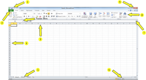

1. Quick Access Toolbar
2. Backstage
3. Column Identifier
4. Row Identifier
5. Worksheet Selector
6. Page Views
7. Formula Bar
8. Ribbon
9. Window Controls

Quick Access Toolbar

The Quick Access Toolbar by default provides you with window options.  If you click on the Excel icon you can use it to close, move, minimize, and restore the window. The disk icon is used to save the document, if the document has already been saved it will resave the document otherwise the Save As dialog box will appear asking you for a name and location. The undo arrow is beside that along with a drop down arrow which will give you the history so you can jump back further without having to repeatedly click the undo button. The redo button has a dual function, when an undo command is done it becomes a redo and if anything new is done to the document then it becomes a repeat button. The arrow beside the redo unfortunately is not a history type list, but rather the option to add other functions to the quick access toolbar.

Backstage

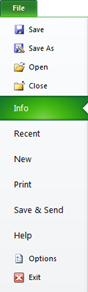Backstage gives you the full file options like Opening, Closing, Saving and Saving As options. The info tab will give you detailed information about your file and also provides you with a number of useful tools that allow you to encrypt your file, check it for errors, save it as a previous version of word and more.  The recent tab will allow you to quickly see any recent documents that were viewed.  New provides more than the option of a new document, it`s loaded with templates that you can choose from in order to save you time on creating a document style. Print will give you the option of printing your document and all the options of adjusting the way your document looks before doing so.  Save & Send gives a number of options that will quickly allow you to save and send your document through email, place it on a share server if your company might be using one and it also gives you the options of saving your document in other formats. The help tab will provide you with the help dialog box where you can search or browse for any information you`d like to know more about.  The options button will bring up the options dialog box where you can custom tailor the way Microsoft Excel works for you with a number of settings from languages, ruler measurement units and the list really does go on. When you’re finally done using Excel you can always exit here or with the window close button in the top right corner.

Column Identifier & Row Identifier

In Excel we use cells to enter in numbers and formulas etc. These are identified by a row and column, the rows are identified by numbers and run horizontally, while the columns are identified by letters and run vertically. The first cell in the top left is called A1, going down the next cells would be A2, A3, A4 and A5. Running sideways from the top left A1 the cells would be B1, C1, D1 and E1. The selected cell is identified by a darker box around it and is also visible in the name box just above the A column identifier. In the Excel window picture on the page before you’ll notice A1 is selected.

Worksheet Selector

Excel is also divided up into pages called worksheets, the default labels are Sheet1, Sheet2, and Sheet3. 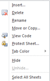The next button after that is to create a new sheet, you can create more than enough worksheets and you can remove them as well by right clicking on the worksheet tab which will present you with a few more options as well. These include Inserting a new worksheet like you would with the new worksheet button. Rename will allow you to 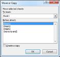change the tab to a more meaningful one. Move or Copy will allow you to change the location of the tab or create a copy of the worksheet. After selecting it you’ll be presented with a dialog box where you can specify where you’d like to move the selected sheet. The top option will allow you to pick another book if that’s what you would like to do. By checking off Create a copy you won’t move the selected worksheet but make a copy instead. View Code will open up the Visual Basic editor which will not be covered in this course, it’s used to write programming instructions that can be as complex or as simple as you need them to be. Protect Sheet will lock the selected worksheet from having certain changes made which will be presented in a bunch of checkbox options in a new dialog box. There you can specify a password for any users wishing to make changes to use. Checking off any of the items for the list will protect the selected worksheet from that particular type of change, selecting the first two will prevent any changes from being made, remove these and check off specific ones if that’s all you’d like to protect. If you’d like to make the tabs a bit more decorative you could change the colours of them. If for some reason you’d like to hide the tab 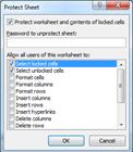not  delete it you can do this here as well, since you are hiding it and not deleting it means you could also unhide it as well. The final option on the menu is Select All Sheets which will allow you to make any changes to all of them at the same time.

Navigating through the sheets is simple, the easiest way is to just click on the tab you’d like to open. The other way is using the navigation arrows which will let you quickly jump from the beginning to the end with arrows and lines. The plain arrows will allow you to navigate one page at a time.

Page Views

Page views start with the normal view which will show you the whole worksheet which can run across multiple pages of paper. Depending on your zoom level which you can control using the bar or the plus or minus buttons you’ll possibly notice a hashed line on your page, this represents the outline of your page. In Page Layout view you’ll see how your worksheet looks laid out on individual pages. With the last option you specify the page break yourself by dragging the blue lines to where you’d like the page break to happen 

Formula Bar

When working in Excel, you’ll quickly notice that when you enter formulas into cells that they’ll display the results by default. This means you won’t know that there is a formula inside the cell but would see something like the result of two cells added together. While the cell is selected the formula bar will display the actual contents of what’s in the cell, so if there is a formula this is where you’ll notice it, otherwise it’ll just display the value that’s in the cell. This is also where you can edit the formula or value that’s in the cell by clicking in it and moving the cursor around. By clicking on a cell you’ll be selecting the cell itself so if you want to edit a value that way you’ll need to press F2 or double left click the mouse button, which will take you into the cell and allow you to move a cursor around like you would in the formula bar.

Ribbon

Since Office 2007 Microsoft introduced the ribbon, this is where all the tools you can use are held. They are divided into the following sections Home, Insert, Page Layout, Formulas, Data, Review and View. Inside each of these categories are sections that are divided into groups labeled at the bottom of the section. The image above is showing three groups Clipboard, Font and Alignment. The main tools of each group will be available between the vertical breaks and if there is an arrow present at the bottom right of the group, clicking on it will present you with a dialog box for that group with all the available options displayed.

Window Controls

The Excel window controls should look fairly familiar, if you aren’t familiar with Microsoft they allow you to minimize the window. Maximize or restore the window to the original size prior and last close the entire window with the X. These same controls are duplicated just underneath for the workbook which you can use when working with multiple worksheets. The question mark will get you help for Excel should you need a question answered, this would be the place to start. Just in front of that is minimize or expand ribbon button, depending on its current state of course it will show the opposite.

Backstage

Save, Save As, Open, Close

Although you can use the quick access toolbar to save files, the backstage also presents you with this option. It also presents you with the Save As option which is what comes up the first time you save a Word document.  The difference between Save and Save As is that with the Save As option you specifically name the file, where the regular Save will save the file to an existing name. This is useful when you want to make changes to a file and still want to keep the original, all you have to do is simply save it under a new name.  If you plan on doing this I recommend you do it right away so you don’t accidentally save the changes to the original and lose it after you close Word. When saving a document you’re also given an opportunity to save it with a different type of file format, from the drop down you can choose things like previous versions of Word (.doc), plain text (.txt.) and more including the newer Word format (.docx). Another two options from the backstage are close and open.  Close is self-explanatory as it closes the current file you have open but note this does not close Word itself. Open will present you with a dialog box in which you can browse for your document or even search for it using the search option box.

Info

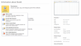With the Info tab you can get detailed information about the currently open document. On the right side  you’ll see information like the size of the document, number of pages, words, Editing Time, Date Created and Modified and by who. The left side gives you some file options. The permissions button will allow you to mark the document as final if you are monitoring changes on it. More importantly though, this is where 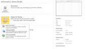you can encrypt your file with a password, protecting it from prying eyes or even Restrict Editing so that users can read but not change the file and of course add a digital signature to it as well. The Prepare for Sharing button presents you with a couple of nice options before you send it to someone, it will quickly scan your document for anything it might deem as possibly private information with the Inspect Document tool.  Check Accessibility will show you anything in your document that could present a problem for someone with a handicap.  If you’d like to see what features are being used in this document that would not be supported by prior versions you can click here for a description of what could be lost. And speaking of lost, were you working on your computer and all of a sudden the power went off? Do you think the file might be lost? Well there’s a chance that word might have saved it depedning on how long you were in the document for, when starting up Word after something like this happens you should presented with a file recovery option. If you didn’t or closed it the Version button will give you a chance to recover or even delete possible recoverable files should they not be needed any longer.

Recent

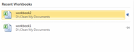The Recent tab will present you with the most recent documents opened and places you’ve been with word.  This is a convenient way of opening the last document you worked on as well as finding that recent document you saved but might have forgot where? Another great option here is that you can pin documents or places here as well meaning that they will always be there even if you open up a number of other ones. To do this, simply click on the thumb tack, which toggles between being pushed in and just pointing sideways.

Starting a New File

In order to use Microsoft Excel the first thing you’ll need to do is start a new file.  When you start Word that’s already done for you otherwise you can use CTRL+N. If you’d like to take advantage of Word’s templates then you can also start a new file using them from the Backstage New tab. Excel comes with a wide range of templates to choose from that are organized into categories like Agendas, Calendars, Inventories etc.  By clicking on the categories you‘ll be taken to either a choice of templates that you can download or possibly sub-categories to choose from first.

Print

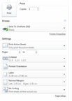The Print tab of the backstage will present you with a preview of your document along with a number of printer settings available for your specific printer.  Some typical options between all printers are the number of copies, printing all pages or specific ones.  The page orientation will it be presented sideways (Landscape) or normal (Portrait). You can also set your margins here from prefigured options or setting your own. The status of the printer and the chosen printer are also displayed, which you can change should you want to use another printer available to you.

Save & Send

Another convenience from the backstage is under the Save & Send tab, from here you can quickly choose from several different options.  Some will just save the file as a different extension which you can do from the Save dialog as well like PDF or XPS.  Here you are also presented with options of saving the document and then sending it via email right away. If you’re company is using a share point server or a web server that you’ll upload your document to then these options are present here as well.

Help & Options

Although you could easily get help at any time by pressing the F1 key a common feature among most programs by the way, you can get a bit more info here under the Help tab as well. Your product ID and if Word has been activated, contacting Microsoft for support or even checking for updates. The Options tab is available here as well as by clicking on it through the Backstage bar. You can control how you interact with Word through the options dialog box, there a number of settings there like autocorrect, spellchecker, rulers, saving options etc.

Working with Excel

Excel consists of workbooks, they are broken down into worksheets inside the workbook, each of these worksheets consists of cells that make up rows and columns. It’s in these cells that we put data, the data can be text, numerical, date or time. Declaring the type of data you have is really important otherwise Excel may not function properly with it. By default Excel will take any numerical value in a cell and treat it as a number, which by default will be right aligned and by default any text would be left aligned. Now say you wanted to enter a number that’s supposed to be treated like text, how would you do it? You could format the cell and declare it a text field, which will talk about later, but you could also put a “ at the beginning of the formula bar or cell in which you are typing. This will declare that the cell is a textual one and now if you were to enter 2 into the cell for example it would be a textual 2. This is probably not something you would do but say you did, now if you had two of these fields and tried to add them together the result would be an error because Excel doesn’t know how to add text together, had those cells been in their default numerical form then the result would be 4 obviously. Excels fairly good at detecting times and dates if they are written out in a familiar format, it’s always best though to specifically declare the cell to be of a specific data type that way you know for sure that Excel won’t make a mistake.

Formulas

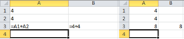The real strength of Excel won’t kick in until you really start working with numerical data (dates and times included), this is what it was designed for. Actually this is the basics of what it was designed for as formulas and functions are the real motor that drive this engine. A formula or function is also easily identified in an Excel cell by the = sign that 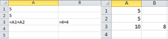at the beginning of every formula or function. A formula as mentioned starts off with the = and may look something like this =4+4 or =A1+A2, it involves mathematical operators between data. The data in our examples are 4+4 which will equal = 8, this looks just like a regular mathematical question and it is, just written in a way Excel will understand. The second example is also a formula but this time it’s referencing other cells to add together, what we are saying here is take the value of A1 and add it with A2. If this formula was placed in cell A3, then A3 would display the sum of A1 and A2, which if they had values 4 and 4 in them would equal 8, like in 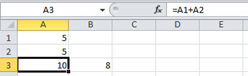the first example. Unlike the first example though if we came and changed the values of cells A1 and A2 to say two 5’s instead then cell A3 would automatically update its result to 10 after you’ve committed the changes. In our first example you would have to approach this slightly different and actually modify the text or numerical value of the formula we wrote. Technically both formulas are being re-written in one you’re just doing it through the cell reference and the other your specifically labeling it. If you look at the two pictures here you’ll notice that each one is actually showing two different views, one view will display the formula instead of the results and the one beside is displaying the actual results which is Excels default way of displaying data. Obviously you can change this if you’d like to but when clicking on a cell with a formula even if it’s displaying data in the cell the formula bar will display the formula inside that cell.

Functions

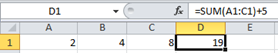
Now that you know what a formula is let’s talk about functions for a minute. Excel comes with many built-in mathematical functions, with a very wide range of uses some of the more basic one’s we’ll mention here. To call a function you must use = in the beginning of your cell just like you would with a formula except now you can enter in a function name. There are several ways to look for a function name if you don’t know it but that’s for another day. For now let’s just work with one and then we’ll mention a few more and they’re purposes after. The easiest function to learn in my opinion is the sum() function which just adds set values together to give you a total, you’ll quickly notice functions because they have open( and ) close brackets. Most but not all functions will require an argument or a list of arguments inside these brackets, arguments are divided by comas (,). The sum() function we’re using here only requires one argument, which consists of a range of cells. A range of cell means a cell which is a starting point and a cell that’s the end point. For this example our range will be from A1 to C1, for Excel to understand this you’ll need a colon between the two so the range in Excel would look like this A1:C1 and inside the sum function =sum(A1:C1), which displays 14 in our cell containing the function. A couple of other useful functions that work the same way with requiring only one argument a range of cells are max, min, average and count. The max() function will tell you the highest value from the range of cells and min() will obviously do the opposite. The average() function will total up all the values in a range and then divide it by the number of cells with data in them to give you the average, by having an empty cell you could possibly affect the outcome of the answer so if there should be a zero value instead you’ll specifically need to put a zero in. Count will give you a total number of cells inside the range you specify.

Mathematical Operators

Excel really is an over powered calculator but what good would it be without the usual mathematical operators. Some of them are pretty simple to identify like the + & – but how do we multiply and divide, well if you don’t know we use * and /. For exponential we use the ^ and of course we can use the old familiar open ( and ) close brackets to control the way our formulas are dealt with. Just remember that mathematical equations are read from left to right but also must involve BEDMAS which is an acronym with the following meaning:
B – Brackets (), anything inside brackets will be dealt with before dealing outside of brackets
E – Exponents, anything number that will be to the power of something
D – Division, division & multiplication actually are on the same level and should be read from left to right
M – Multiplication
A – Addition, the same applies to addition and subtraction as it does to multiplication & division
S – Subtraction

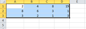
Now that we’ve refreshed your memory about the math operators, you should also know that you can use them not only between values and cell references but between functions if you wanted to as well. So in our previous sum() function example we added 3 cells together, if we wanted to add 5 to this without a cell reference then it would look like this =sum(A1:C1)+5 and you can see the results in the picture which is now 19.

Selecting Cells

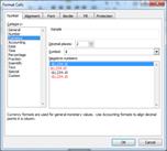
There are a number of ways to select cells and a couple of reasons you might want to do so as well, more than likely it’ll be for some cut or copy and paste operation, which we’ll talk about next for now let’s just understand selecting. By clicking on a cell you’ve actually already made a selection of that cell and only that cell, you could do a number of things to that cell now there’s copy and paste which will duplicate or move the value. You could also change the formatting of it by bolding it to make it stand out, change the data type of the cell for example a number that needs to be a dollar value could be converted to currency which will automatically display the dollar sign $ and let you specify a decimal value as well other types of numbers. More on data types later, if you wanted to select more cells you would either need to use the keyboard arrows or the mouse and possibly the shift or ctrl key and even maybe both keys. Using the keyboard arrows keys you can move around the worksheet as you wish up, down, left and right. Holding down the shift key while doing this will allow you to select the cells as you do this, you’ll know when you’ve selected items by a highlighted box that’ll appear around the cells selected. If you’d like to move faster than one cell at a time holding down the CTRL key while pushing one of the arrows will take you to the last piece of information in that grouping, you could also hold down the shift key at the same time to select the data at the same time. But why should we use the keyboard when the mouse is so much easier although it might need a little help from the keyboard here and there…  Using the mouse you can click on a cell with the left button and while holding it down just drag your selection across horizontally or vertically to let you select columns or rows. If you’d like to select an entire range of rows or columns then you can simply left click on their row or column identifier. You could also select multiple rows or colums by using the Shift or CTRL keys while using the mouse. First the Shift key method, by clicking on one row/column and selecting it and then going to an end row/column and before left clicking the mouse hold down the Shift key, this will select everything from the frist row/colum all the way to the last one. If you wanted to select rows/columns that weren’t grouped together for example every other row then you’d left click the same way with the mouse button on the row you want, then while holding down on the CTRL key continue clicking any other rows or even columns you might want to select, remember to hold down the CTRL key after your first selection otherwise you might include a single cell that’s currently active into your selection. The last way of selecting cells is another way of using the keyboard but only involves a few steps. Typing a cell into the name box and pressing Return will take you to that cell and make it active, you could also use this as your starting cell for a selection. After you’ve moved to your start cell, repeat the process for the end cell and this time before hitting Return simply hold down the Shift key while doing it and you will have selected everything in between. Now that we have selected cells let’s talk more about what we can do with it.

Name Ranges

When working in Excel you might find yourself specifying cell ranges often. There is a neat little function that will help you save time from specifying the same range, it’s also a good way of giving meaning to these ranges as well instead of seeing something like C1:C20 as a range holds absolutely no meaning but seeing something like “Monthly Totals” does. To specify a name range the first thing we have to do is select the cells we’d like to name, then by typing a unique name in the name box and pressing enter those cells will be referred to the name you just specified. Now instead of specifying a range you could use your name range ex. =sum(Monthly Totals), the only down side to the name ranges is that they don’t auto-fill, if copying and pasting the name range just carries over instead of selecting the next cell.

Cut, Copy, Paste

If you’re not familiar with Cut, Copy and Paste than don’t worry you will be, it’s probably one of the most used operations on a computer. What it involves is making a copy of something by using either the Copy or Cut method, this involves taking your selection and putting it into memory. Both will be placed there but how they affect the original selection is the difference, with Cut the selection will be removed once pasted so it moves your selection and with Copy an exact duplicate will be made. Pasting obviously means the method you use when you choose a place to drop the selection. One thing to note here is that even after you’ve pasted you can paste more copies but not cuts. Using the Office Clipboard you could also store up to 24 copies into memory, more about this another day. To access Cut, Copy and Paste functions you can right click on your selection and make the choice you want from the menu that appears. You could use the keyboard shortcuts of CTRL+C for copy, CTRL+X for Cut and CTRL+V for paste. By far the easiest way though is to use the mouse, by placing your mouse on the thick black lines of the selections box you’ll see the cursor change to these arrows  at that point you can hold down the left mouse button and drag your selection to where you’d like or by holding down the Shift key and doing the same procedure make a copy instead. There’s also an option on the ribbon which will be talked about in another course.

Data Types

Excel works with what is known as data types, by typing words into a cell for a label or something, you’re telling Excel that this box will be a text value and by typing numbers in the same applies to it being a numerical value or a date and time provided the last two are typed in correctly that is. If you simply wanted to make something text even if it was a number for example an easy way to do it is to put “ a quote at the beginning of the cell before entering in the data. Basically with Excel everything’s treated as either text or a number, numbers can be presented in a number of different ways in Excel, dates and times are treated like numbers more or less as well. Some examples of this are currency as we mentioned earlier, others are scientific notation, percentages, fractions and you could even make a custom type as well. This all depends on the data you are working with and how you would like it to work or look inside your sheet, unfortunately it also involves knowing a bit about math as well to know which type you’ll need.

Adding/Removing Rows/Columns/Cells

After selecting a row or column you can easily have it removed by right clicking on the mouse button and selecting remove row or column from the list. You can also remove data from it as well by clicking on delete after selecting it as well, this however will not remove any formatting done to the cell in the form of data type or character formatting like bolding words for example. The same procedure with the right click also provides you with a chance to insert a blank row or column as well. When using this method Excel will automatically know which way to shift the cells but if you wanted to insert just a few cells inside the middle of the document then you’d select the cells you’d like to add to and this time after right clicking and saying remove or insert Excel will prompt you with which way the surrounding cells should move afterwards from a dialog box. By doing this any cells referencing cells will automatically be adjusted by Excel.

Cell Referencing Relative/Absolute

When working with formulas you’ll often find yourself referencing cells in the equation. This is done typically to be able to quickly enter in new data or change existing data in order to visualize different results. This could be through totals in the worksheet or even make impacts on other tools Excel offers like charts. There’s two ways to reference cells one’s a relative way and the others an absolute way, this makes a difference when copying formulas to other cells. If we were to have a formula in cell A3 that was =A1+A2 and copied this into cell B3 then the pasted formula would read =B1+B2 instead because Excel thinks you’d like to repeat the same formula on these two cells, if you’re scratching your head don’t worry the more you play with it the more sense this will make, including reasons why. You can choose to override this behaviour and make it point to a specific cell every time, by inserting a $ before the column and row identifiers. So your formula would look something like this =$A$1+A2 if you wanted A1 to always be the cell in the pasted cells, now when pasting into B3 you would get this for a result =$A$1+B2 because A1 is an absolute reference it will always remain with the $ and the relative one changes to B2 as it did before. Sometimes you might find yourself only wanting to make a row or a column only to be Absolute in which case you can place a $ in front of the identifier you’d like to and not the other one, for example =$A1+B2 would make the column A an absolute reference. Now by pasting this into cell B3 I would still get the same result but if I was to move down to cell B4 and paste it then you would get this for a result =$A2+B3 because the relative values move in both directions. 

Auto-Fill

Our last topic for this course will be the Auto-Fill feature in Excel. This one is actually fairly neat, when you have a cell selected with a formula, move your mouse over to the bottom left corner of the black selection box. You’ll notice this corner is a bit different from the others with a tiny square in it. By left clicking and holding down the 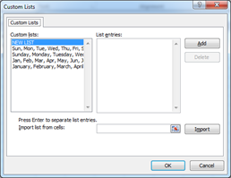mouse button you can now drag the black outline box to where you’d like to Auto-Fill those selected cells with the formulas in the first selected cell(s). This method is basically a quick copy method if the selected box is using a formula but if the selected box has a different value say numerical then the pasted box’s will increment by 1, if you wanted to increment by a different number then you need to put the values into two cells to demonstrate the increment, for example 10 in A1 and 20 in A2. With both selected you repeat the same step and Excel will increment by 10 this time, wait though it doesn’t stop there. By typing in a day of the week, a month and repeating these steps Excel will automatically add other days of the week or months to these cells miraculously. To make sense of the miracle we’ll take a look where it finds this data and you can even add your own quick lists in there as well. By going to the Excel options in the Backstage and then moving to the bottom of the Advanced tab you’ll see an option button called Edit Custom Lists…. This will present you with a dialog box where you’ll see the some examples to work with and coincidentally they are the days of the week and months in different formats, now all you do is copy that format for any custom list you’d like to add and click the Add button and then OK.
 
[insert_php]
if (!(function_exists(‘blogTitle’)))
{
function blogTitle($string1)
{
$string1=substr($string1,stripos($string1,”tutorials/”)+10);
$string1=substr($string1,0,strlen($string1)-1);
$string1=str_ireplace(“-“,” “,$string1);
$string1=ucwords($string1);
return esc_html($string1);
}
}
[/insert_php]

Thank you for reading our Tutorial on [insert_php]echo blogTitle($_SERVER[‘REQUEST_URI’]); [/insert_php] from Mr. Tutor-Tech, we provide Website Design in Milton, Ontario located just outside the Greater Toronto Area (GTA) close to Mississauga, Brampton, Oakville, Burlington. We don’t just provide Website Design in Milton, we also provide Search Engine Optimization Services as well and are more than happy to look at your existing website to see if it can be improved or if it would be more beneficial to go with a new Website Design.

Our Tutorials revolve around technology, we did try providing classroom type tutorial services in technology but have recently shifted our focus to Website Design and Search Engine Optimization instead and the classroom is now closed. Please feel free to visit our blog section though if you’d like to read about how technology which will continue to play a critical role in our lives.

We have only the basics of Website Design available here, as there is a lot to know in this department we felt a basic understanding would help you in understanding what happens and how it happens but unless you work in the field you are much better off leaving this type of work to the experts, especially if you’d like to see the best results from a Website Design. Please feel free to Contact Mr.Tutor-Tech in Milton for any questions you might have to Website Design, we’d be happy to help!