Microsoft Excel Level 2

Table of Contents

Formatting

When working with Excel 201 there’s two types of formatting, we briefly touched upon both of them in the previous course. They’re the data type format and style format, the data type format refers to if the cell contains text, numerical value, date or time, etc. When we make the data look pretty or stick out in a particular way then we’re referring to the style of that cell. Most of these functions are found on the Home tab of the Ribbon.

Home Tab

Clipboard Group

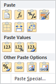Before we get into formatting we’ll talk about the first group of the Home tab the Clipboard, you should already be familiar with copy and paste from our previous course or possibly some other program. Along with the few options we’ve discussed in the previous level you can also copy, cut and paste from this group. Cut is pretty much standard and the same as before but with copy we have an additional option in the drop down menu and that’s to copy as a picture. This will allow you to paste the selection as an image in other programs or even in Excel which will allow you to manipulate it as well, special effects, changing angles and more. The Paste drop down offer short cut options for the paste special which gives you more power over what will be pasted, the menu many vary depending on what you have copied to memory but they may include:

Paste

• Paste – This is your typical paste option which includes formulas and formatting
• Formulas – Will just paste the numerical and formula values
• Formulas & Number Formatting – Will paste formulas along with numbered formatting
• Keep Source Formatting – Will paste with the formatting from the source
• No Borders – Will paste without any borders if the source included some borders
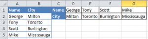
• Keep Source Column Widths – Will keep the source column width Transpose – this will flip your selection and is used to change table from running vertically/horizontally and switching it in the other direction

Paste Values

• Values – This will just paste the values and not any formula or formatting
• Values & Number Formatting – Use this if you’d like to retain the data formatting
• Values & Source Formatting – Use this if you’d like to keep the source formatting

Other Paste Options

• Formatting – This will paste just the formatting from the selection and is basically the Format Painter which we’ll talk about in a second
• Paste Link – This will paste links to the original cells
• Picture – This will paste it as a picture allowing you to use picture adjustment tools
• Linked Picture – This will also paste as a picture but any updates in the original will reflect the changes in the picture

Paste Special

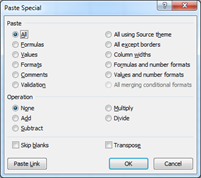Should one of the previous combination not work for you then you can come up with your own by clicking on Paste Special you’ll be presented with a dialog box with some of the familiar options mentioned above. Two new options are Operation and Skip blanks. Skip blanks will allow you to leave the values in the destination intact if the copied area is blank. The Operation area allows you to choose from Add, Subtract, Multiply and Divide, these will applied against the numbers of the destination area with the numbers from the source.

The Format Painter is a neat little tool which allows you to copy the format from one cell and quickly paste it to other cells. With the cell you’d like to copy active click or double click on this tool and simply just go to the destination cell and click again, if you had double clicked on the tool then it will stay active and you can continue on pasting until you click on the tool button again, if you only clicked once then don’t worry it’ll deactivate right after you paste your first selection.

Font Group

The Font group is the first group you can use to format your data, with this group you can change the font from the box in the top left simply by selecting the desired font from the drop down list. You can make the fonts or smaller by selecting it’s size from the next drop down list or by using the two boxes beside it with the bigger and smaller A, this will increase or decrease the font by the points available in the list. Starting the next row is B button for bold, I button for Italicize and U for Underline. The next button will give you a drop down and allow you to choose what type of border you’d like to apply to the selection. Here you can specify from a particular side, all sides, outline and no border. They each also act as a toggle so they will add and remove that particular selection. You can also choose from different types of lines along with thickness and colour as well. The last two options allow you to change the background colour and font colour from the options available, along with 16 million or so combinations available through more colours.

Alignment Group

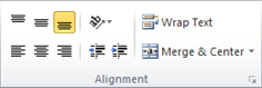The Alignment group gives you several options on how you’d like to align your data, the first top three buttons allow you to specify vertical positioning and the bottom three horizontal positioning. Next we have the Orientation tool which will give you a drop down of options along with the Format Cell Alignment option which will present you with a dialog box with more specific control of what you’d like to do. Just underneath that are the decrease and increase indent buttons which will adjust your text according to the one selected. When displaying data in a cell Excel will by default let that information run outside of the cell range and into other cells, if you’d like to prevent this and have the text stop at the end of the cell and continue on the next line then you’d select Wrap Text. On other occasions you might want to merge several cells together for example when giving a table a title or something like that, this way the title cell starts and ends with the table by using the Merge drop down button you can not only merge cells together but you can separate merged ones and also apply formatting while merging by specifying Merge & Center. Merge Across will join cells to already merged cells.

Number Group

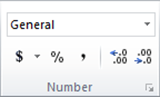There are a number of different data type formats available in Excel, the Number group is where you specify what selected cells will be. With the first drop down list you can select from a number of the most common types available, there are basically three groups, numbers, text and date & time which typically are grouped together. There are a number of different numerical types some include currency, number (decimal or whole), percentage and more. The one you choose really depends on your data and the look you might want to give your report, to many decimal places might look ugly so maybe you’d like the results rounded off to the first one for example. A few other options presented in this group are the Currency button with a drop down of different types of currencies, percent or coma separated numbers for easier reading. The next two buttons will allow you to specify more or less decimal points visible.

Styles Group

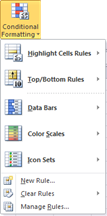The Styles group lets you control the look and feel of your excel sheet. The first button Conditional Formatting is a little more complicated compared to the other tools in this group.  It’s not difficult to use but requires some understanding behind what it does. By clicking on the button you’ll be presented with a drop down which you can choose several different conditions from. Conditions reflect the data that’s being presented, with Highlight Cell Rules you have several options to choose from, the first four compare the data to the rules you specify. The first two will highlight numerical values that are higher or lower than the values you specify in the next dialog box. Where you also specify the colour you’d like to use to highlight those cells. The next two boxes work much in the same way except it’ll highlight numbers that are between ranges of numbers you specify or equal to the value you specify. Top/Bottom Rules is a quick way to have the top 10 or bottom 10, top 10{463c70c279fb908728b910a090d44fbe4ae7aabcd875de9c1a518a8c8e2be8bd} or bottom 10{463c70c279fb908728b910a090d44fbe4ae7aabcd875de9c1a518a8c8e2be8bd} of your values highlighted, you even have the option to highlight above or below average data here. Most of these submenus also have the more rules option at the bottom, these will give you a bit more control of your rules should you need it. These include styling options along with more control of say something like top 10 and you’d like 20 instead. Data Bars gives a very nice representation, it’s like a chart in the background, it’ll take the values and shade their cells so that the least and most are either full or empty and everything between will have a bar reflect the differences in between.  You can make either low numbers or high numbers stand out here so that the highest number for example will have complete or no fill and the low number would be the exact opposite, for this you need to enter the more rules option otherwise the chart will show lowest number as empty and highest number as full. Color Scales and Icon Sets work in much the same way as the Data Bars except they either give a range of colours from lowest to highest like blue for low and red for high or a graphical representation with Icons like a down arrow for low and an up arrow for high.

The Format as Table button does a little more than just give a style to your table. With this button the data you have highlighted will also be converted into a table if it already isn’t one. A table can be entered in one of two ways as all data with no header information or with header information, if you haven’t converted your data to a table you’ll receive a dialog box allowing you to do so, this will allow you to highlight the data if you haven’t before clicking as well. Note the checkbox My table has headers, if you have header information selected check this off. 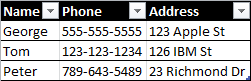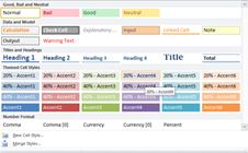A good example of a header is a phone book with the words Name, Phone Number, Address written at the top and data under that, it allows you to easily know what the data is. Along with the styling of the table like shading every other line and accenting the header information you also get a few controls placed on your table as well, you’ll notice the arrows in the picture beside each column. These allow you to sort or filter those particular fields to remove useless information or make it more manageable to read, like alphabetical by name. Some of this will be talked about in the Editing group in a little bit, we’ll concentrate on filtering for now. The filter option allows you to remove unwanted data by removing checkboxes from the data at the bottom of the drop down you’ll hide that information you can also use conditional filtering by clicking on text filters or number filters (depending on the data selected you’ll receive one of these options). Here you can look for data equal to, higher or lower (numerical), values that start with a certain value or values that don’t have a certain value and more with the custom filter option at the bottom.

The Styles box allows you to manually give visual effects to your spread sheet simple clicking on any of the styles available will format that cell to make it look like the style selected, this includes both highlighting and font styles depending on your choice, by clicking the second down arrow you’ll also be allowed to choose from more styles available not to mention Merge Styles or create New Cell Styles of your own. 

Cells Group

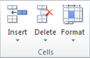The Cells group is fairly easy here you can you can add or delete cells, rows, columns or sheets with the Insert button and the Delete button. Remember you can also do this by right clicking on the cell or column identifier or highlighted/single cells as well. The last button here Format allows you to control the width and height or your cells selected. You can specify what you’d like or have it atomically done for you. You can also hide/unhide data from your worksheet, allowing you to remove data but not delete it. Using Organize Sheet options you can rename your sheet, move or copy others and give the tab at the bottom a color style. The last few options allow you to lock cells to protect your data which will be talked about in another level for now just know that it’s here. A secondary spot for formatting cells is also available here should you want to convert a number to a dollar value for example.

Editing Group

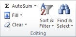The Editing group starts off with a very nifty tool the AutoSum tool, which acts as other Auto tools as well by clicking on the arrow you have the options of selecting Sum, Average, Count Number, Min and Max values. This tool will automatically highlight the values it thinks it should use but you are free 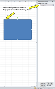to give it a new range and will perform the appropriate calculations based on your selection. At the bottom is the option for more functions as well should you want to perform some other type of calculation. The fill drop down allows you to take one cell and have its information copy over to the cells in the direction specified. You can also take care of auto increments here so that each new cell will increase by a certain number the default is to add 1. The Clear button allows you to remove data, formatting, comments, hyperlinks or all of them from the cells selected. The Sort & Filter button gives you the option of sorting the selected data it also turns on/off the filtering options given on the table discussed earlier, by checking the Filter button you’ll toggle this option on and off, there’s also an easy way to clear all filtering here with the clear option. The Find & Select button allows you to search for certain text, you can also use it to replace certain text through your sheet as well. Using the Go To options you can jump to a particular spot inside your work sheet like a certain cell or a named range, you can filter this option further by specifying the type of data you’d like to jump to using the Go To Special or the shortcuts (Formulas, Comments, Conditional Formatting, Constants) for data types just underneath. The Select Objects and Selection Pane allow you to easily work with the different objects you inserted into your work sheet like clipart or an image. This freezes your Select Objects freezes your data making it easy to just select these objects and the Selection Pane will list all these objects inside of it so you can quickly see what you have and jump to it.

Page Layout Tab

Themes Group

The first group in the Page Layout tab is Themes here is where you control what font types and colours will be used in your spreadsheet. Unless you have colours in your spreadsheet you won’t notice this change but you will notice the fonts change as you hover over the different themes. When selecting colours for a background if you select from a theme colour these will adjust as you hover over the different themes. The Colors button allows you to choose the colour groups you’d like to use in your theme and will be reflected inside of your options for filling in cells. Fonts let you choose the group of fonts you’d like to use inside your sheet. You’ll notice there are two fonts associated with each selection one’s for headings and the other for body, depending on if a style was applied to your sheet or not you’ll see differences as you hover over the different choices, don’t forget your free to make up your own combinations of fonts and colours. The Effects buttons applies to objects drawn inside of Excel and will apply your choice to them.

Page Setup Group

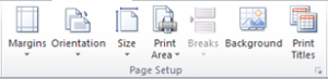The Page Setup group allows you to adjust the way your data will appear on printed pages. The first button Margins allows you to specify your margins, which is the white space around the border of your page, top, bottom, left and right. You are free to choose from the 3 pre-sets here or you can specify your own should that not work for you. You can also adjust your page to be horizontal instead of vertical by clicking the Orientation button, the default page setup is portrait but you have the option to convert it to landscape which will use your paper sideways. There are a number of options available under Size as paper isn’t one size fits all, here you can select from a number of pre-sets the default is letter 8 ½ X 11 but you can choose legal, envelopes or set your own for custom paper sizes. The Print Area button is used to either clear or set print areas, you can use this to start a new page on paper, a good example would be to keep groups of data together, so if you had something like a North Office with 10 locations but 2 were going to display on the page before you could set a new print area forcing all the office locations to be together on the next sheet. You can use Page Breaks pretty much for the same purpose as the print area by forcing a page break you tell Excel you’re starting a new page at this point, here you also have the option of removing the break or clearing all of them at once. 

Scale to Fit Group

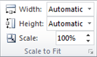In the Scale to Fit group you have a few options in regards to how much data you’d like to fit on a sheet, here you can control how much data will fit either the width, height or both. Scale will adjust your data by shrinking or expanding it according to the percentage you specify 100{463c70c279fb908728b910a090d44fbe4ae7aabcd875de9c1a518a8c8e2be8bd} being the normal view. The Width and Height dropdown lists allow you to tell Excel that you’d like to fit all the data across the amount of pages you specify either height or width wise depending on your choice. Usually this involves shrinking your data so be careful not to overdo it as you might not be able to read the information off of your printed material.

Sheet Options Group

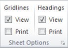The Sheet Options all you to tell Excel if you’d like to view either the Gridlines or Headings inside of Excel itself by checking or clearing the view checkbox. You can also specify if you’d like to see these on printed paper as well, the headings is referring to the numbers and letter used in Excel to identify a cell and Gridlines are the lines you see in between the cells in Excel. If you find this annoying for some reason this is where you go to have a clear page.

Arrange Group

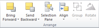The Arrange group allows you to manipulate inserted graphical objects on your sheet. Bring Forward and Send Backward work only when there are multiple objects on your sheet. They control which one will be on top or bottom should you want to overlap them. The Selection Pane will open up a pane showing you all the objects in your worksheet, making it easy to jump to and select the different objects. Align mainly works with multiple objects selected, here you can quickly align them from left to right or centered horizontally or top to bottom and centered vertically. With more than two objects selected you can also 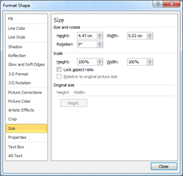evenly distribute them both vertically and horizontally. By turning on Snap to Grid or Snap to Object you’ll quickly be able to align your objects to the selection made, these are toggle options so you come here to turn it on or off. The last option is the same as the one from the Sheet Options group where you can turn on or off the gridline’s. With more than one object selected you’ll be presented with the Group button this will combine them to one so that you can make changes to them together, by selecting a grouped object you can also ungroup it from the selection presented in this menu, once you use this you also have the option of regrouping. The last option in this group is the Rotate button which does exactly what it sounds like it does, which is allowing you to rotate that object you selected by 90 degrees at a time or completely flipping the object either vertically or horizontally. If you’d like to more control over the degrees of rotation then simply select the More Rotation Options, here you’ll get the Format Shape dialog box and be able to not only specify the degrees of rotation but adjust or scale the image as well.
 
[insert_php]
if (!(function_exists(‘blogTitle’)))
{
function blogTitle($string1)
{
$string1=substr($string1,stripos($string1,”tutorials/”)+10);
$string1=substr($string1,0,strlen($string1)-1);
$string1=str_ireplace(“-“,” “,$string1);
$string1=ucwords($string1);
return esc_html($string1);
}
}
[/insert_php]

Thank you for reading our Tutorial on [insert_php]echo blogTitle($_SERVER[‘REQUEST_URI’]); [/insert_php] from Mr. Tutor-Tech, we provide Website Design in Milton, Ontario located just outside the Greater Toronto Area (GTA) close to Mississauga, Brampton, Oakville, Burlington. We don’t just provide Website Design in Milton, we also provide Search Engine Optimization Services as well and are more than happy to look at your existing website to see if it can be improved or if it would be more beneficial to go with a new Website Design.

Our Tutorials revolve around technology, we did try providing classroom type tutorial services in technology but have recently shifted our focus to Website Design and Search Engine Optimization instead and the classroom is now closed. Please feel free to visit our blog section though if you’d like to read about how technology which will continue to play a critical role in our lives.

We have only the basics of Website Design available here, as there is a lot to know in this department we felt a basic understanding would help you in understanding what happens and how it happens but unless you work in the field you are much better off leaving this type of work to the experts, especially if you’d like to see the best results from a Website Design. Please feel free to Contact Mr.Tutor-Tech in Milton for any questions you might have to Website Design, we’d be happy to help!