Microsoft Excel Level 3

Table of Contents

Insert Tab

Tables Group

The first group available in the Insert tab is the Tables group and the first button presents you with the option of selecting a Pivot table or Pivot Chart. These tables and charts can be a bit complicated and will be talked about in another level. The next button available in the Tables group is the Table button, by clicking this you’ll be prompted for information regarding the range of cells that create your table. This is the same dialog box you get when using Format as Table from the Home tab talked about in the previous level. By creating a table you’ll be able to apply styles to your table as well as be provided with arrows for sorting and/or filtering each column in your table. An additional tab will also appear to help you style or change your table.

Table Tools Design

Properties Group

The Properties group allows you to give a meaningful name to your table, which you can use in such things as the go to tool. The second options available here is the Resize Table, which actually sounds kind of deceiving. You’d think you’d be able to shrink and expand your table with this tool but that’s not what it’s for, it’s here to let you specify the data that will create your table, useful if you added or deleted some data from the original table.

Tools Group

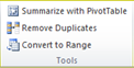The Tools group offers three functions, the first one being Summarize with PivotTable which creates a PivotTable from your table, more about PivotTables will be covered in another level. With the second function Remove Duplicates you can tell Excel what data to look at it by checking off their appropriate checkboxes and then after clicking OK any duplicates will be removed. Convert to Range will turn your table back into an ordinary range which is how it started, this will also remove the filtering and sorting capabilities available through a table. You can still sort ranges, just won’t be able to filter them.

External Table Data Group

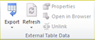The External Table Data group allows you to work with information coming from another source like a SharePoint server. This tool will only be available with external data and will not be covered.

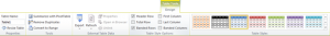
Table Style Options Group

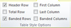
The Table Style Options group has several checkboxes in it which let you display or highlight certain parts of the table by checking them off. The Header Row will hide or show the header information by checking it off, same as the Total Row. Banded Row, First Column, Last Column and Banded Columns all will accent those particular rows with a different colour.

Table Styles Group

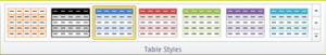The Table Styles group is pretty much what you see is what you get kind of thing, this is where you pick the colours you’d like to be used in the table. It’s also where you go to clear existing styles or to create your own, by clicking New Table Style you’ll receive a new dialog box. With the dialog box you can set the styles for each of the different options for the table like first row, last row, total etc.

Illustrations Group

Picture, Clip Art & Screenshot

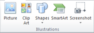
Each of the buttons in this group allows you to add art to your spreadsheet. I’ve grouped these three because they all add the same Picture Tools Format tab to the ribbon. The other two have their own, although they all introduce the same new tab to the ribbon each one of these has a slightly different purpose. The Picture button allows you to add images such as .jpg, .png and .gifs to your spreadsheet. When clicking on the Clip Art button a Clip Art pane will open to the side of your screen. Here you can type in a keyword to search for a specific type of clipart or just leave it blank and click Go to some default ones. You can filter these by their media type with the drop down menu and by checking off Include Bing content you’ll search for extra art not installed on your computer but available via the net. To add a clip art image to your sheet simply double click it or drag it over to where you’d like too. The last button that includes the Picture Tools Format tab is the Screenshot button this will present you with a drop down button with a small image of all the windows that are open on your computer except Excel of course, by clicking on any of these you’ll drop a screen shot of that image into your spreadsheet. At the bottom you’ll also notice a Screen Clipping option, after clicking this Excel will minimize itself and you’ll be able to use your mouse to highlight the part of the screen you’d like to take an image from.  Now that we’ve talked about what these three buttons do let’s move on to the toolbar they all have in common and the functions which can be used.

Picture Tools Format Tab

Adjust Group

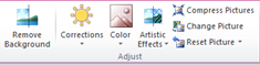When adding any of the types of images mentioned or simply by selecting an existing one the Picture Tools Format tab will appear, here you have several options available to manipulate that art. The first group Adjust offers you several tools for formatting your images. The first one Remove Background is a 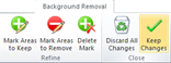tool that will highlight in pink what it thinks it should remove from your image, by clicking the Remove Background button you’ll receive a new temporary tab labeled Background Removal. Here you’ll have the options of adding marks for areas to keep and to remove along with the option of removing those marks should you make a mistake. The last two buttons will either keep the changes you’ve just made or discard them. The Corrections button will give you two options Sharpen & Soften along with Brightness & Contrast, you can choose from the pre-sets available or if you want something more specific you can click on Picture Corrections Options and manually enter the values. The color option has pre-sets that have colour variations should you want to add a tinge of blue or cyan etc. If you don’t see the colour choice available you can always select More Variations to choose from. Set Transparent Color will give you a tool to select a certain colour with, this will make any colours in your image of the same shade transparent. Artistic Effects give you a few special effects to choice from, all of which have a completely different look and feel to them. Compress Pictures allows you to quickly shrink the file size of your image, this will also affect the quality of the picture as well to a dagree, meaning it depends on how you view your content. Most images have low quality and look fine on the screen but not so much when printed. If you’d like to switch the picture with another one then Change Picture is the button you need to click, the dialog box will prompt you for the image location after pressing it. Finally if you’re not happy with the changes you’ve made you can always press Reset Picture, whose drop down menu presents you with two options first one is to reset the picture itself from any changes except size change and the second will reset the size as well.

Picture Styles Group

The Picture Styles group starts off with a box with several choices that give your image a border or other picture effect. You can choose from the pre-sets or create your own specific type with the use of the Picture Border and Picture Effects buttons, which allow you to choose the colour and type of effect you’d like to use. The last button in this group Picture Layout allows you to choose from several different templates which will put your image in a container from your choice and also provides SmartArt type of captioning to this image.

Arrange Group

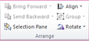The Arrange group has a few options available here and are the same as the one’s provided on the Page Layout tab. The first two buttons Bring Froward and Send Backward require multiple images, what they do is exactly what they sound like they do, either put a picture behind another or bring it forward and on top of the other, depending on your choice. The Selection Pane will open up a window pane on the right side of the screen which inside all image object types for that worksheet will be presented you can quickly select them using this tool instead of scrolling through your spreadsheet. The Align button requires a couple of images to be selected for most of its menu and even 3 or more for distribute options. This will quickly allow you to align images to one another so that you can have it precisely centered for example.  The last couple of options will toggle that feature on and off, Snap to Grid and Snap to Shape will make your image align to the grid or another image when it’s close to one of these edges.  View Gridlines will turn off the gridlines inside your worksheet so that it’s not displayed on your monitor.

Size Group

The last group available on the Picture Tools Format tab is the Size group here you can control the size of your picture by entering new Height or Width inside of their text box’s. You can also use the Crop button to just crop your image normally or to a particular shape and even Aspect Ratio. There’s also Fill and Fit options which will automatically try to make the picture fit keep it’s ratio, with Fill anything that doesn’t fit will be cropped off the picture.

Shapes

Drawing Tools Format Tab

With the Shapes button you’ll be able to select from a number of different types of shapes through the drop down menu, once you’ve selected one of them, go to your spreadsheet and by holding down your left mouse at a starting point and then dragging it outwards you’ll create the shape selected and size it as well. From there you’ll have the option to manipulate the shape using Excels Drawing Tools Format tab.

Insert Shapes Group

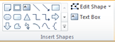The first box in the Insert Shapes group allows you to select and add more shapes to your spreadsheet, just as before simply choose the shape and then left click where you’d like to place it and drag out to the appropriate size. Don’t forget that you can also adjust the location and the size of the shape afterwards as well. Simply grabbing onto the handles that surround the object you can hold down the left mouse button and drag it in our outward to increase/decrease the size of the shape. Depending on which handle you grab you’ll be either able to go either vertically or horizontally and the last option is from the corners and angle wise this will keep the aspect ratio of your shape intact if you hold down the shift key. The green handle can be used to rotate your shape and in this case the yellow handle can be used to give more or less of the page fold that this shape has. The Edit Shape button will allow you to change the shape from the list provided or edit the points of the shape manually. To add text to your shapes or if you’d like to place text in a specific decorative way on your spreadsheet then you use a textbox, simply draw the box to desired size and then enter text inside of it.

Shape Styles Group

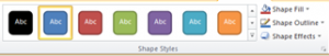The Shape Styles group starts off with a number of pre-set options for you to choose from, they include different shading, fills and outlines. You can also specifically address any of these areas by selecting Shape Fill, Shape outline or Special Effects and using their menus and sub-menus to change the particulars of the shape.

WordArt Styles Group

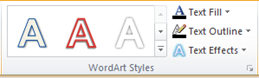With the WordArt Styles group you have control over your text in textboxes and can make them pop out with by giving them colour, fills and other effects. From the pre-sets you can choose from several ones that will reflect your theme and just like shapes you’ll have the option of manually changing the Text Fill, Text Outline or Text Effects using their menus and sub-menus. You can also specify a picture or a gradient using the Text Fill button and with both effects buttons from Shapes and WordArt can apply more than one effect, just not within the same grouping. Also if you’re applying a gradient choose your colour first as choosing it after will set it to a flat colour.

Arrange Group & Size Group

These two groups are exactly identical to the Picture Tools Format group so please refer to them 

SmartArt

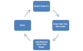
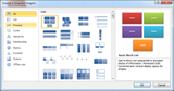SmartArt is a graphical representation of a certain process, hierarchy, cycle etc. By clicking on Smart Art a dialog box will appear where you choose from categories what type of graphical representation you’d like to have, don’t mind the amount of groups that are available to the graphic as you can increase or decrease the amount afterwards. Once you’ve selected your option you’ll notice your image appear on the screen with the words Text written in each of them, by selecting the textbox you’ll be able to write your own text and do this for all the textboxes that you want. If you want extra text boxes or to remove some then you can click on the left right arrows to the left of the image, this will expand the box and provide you with more options. You’ll notice the text you typed appears here or if you haven’t they all say Text. You can change the text from here as well and by hitting enter after each one will move to the next or create a new one. Simply click on any of them and delete the text to remove it. There are also two new tabs that come with SmartArt which are very similar to the ones that you’ve seen with other types of images we talked about, they can help you adjust your SmartArt so it’s just the way you’d like to see it.

Charts Group

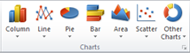With the Charts group you can quickly give your data a graphical representation and you have a wide variety to choose from, the main categories are Column, Line, Pie, Bar, Area, Scatter and Other Charts. Each of these provides you with a drop down menu to choose from a number of styles available. Without any data selected Excel will try it’s best to determine what data on the current spreadsheet it should use, this might not be what you expect so it’s best to highlight the data first before clicking on any of the Charts button. At the bottom of each of them is the option for All Chart Types which will give you all the available options. We’ll be discussing charts in more detail in another level.

Sparklines Group

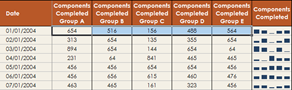With Sparklines you can give your spreadsheet a graphical representation broken down so that there are multiple graphs like for a manufacturing process for example. Let’s say there are 5 groups that manufacture products inside your factory and you’d like to see how they fair against each other or even per day by changing a few options in the new tab you receive when activating or selecting a sparkline. To do this first you need to select the data like we have in the picture above, from there you click on the type of sparkline you’d like. For our example here we’re using columns. We’ve also changed an option on the axis point to have it compare against the highest and lowest points from all the data, by default the sparkline will show you the highs and lows of the data selected. Once you selected the type of sparkline you’d like you’ll be prompted for the destination information, in our example here it’s the cell just after the selection which already has the sparkline in it. After that’s done you can simply copy and paste the sparkline to the cells below. We’ll talk about some of the other options available with sparkline with its new tab that appeared the Sparkline Tools Design tab.

Sparkline Tools Design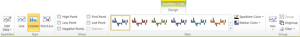

Sparkline Group

With this group you get the Edit Data button which will present you with a dropdown menu. The first option Edit Group Location allows you to edit the range the group data is being pulled from, to change a single sparkline click on Edit Single Sparkline’s Data to do so. By clicking on Hidden & Empty Cells you’ll be able to choose from gaps or zeros to represent hidden or empty cells.

Type Group

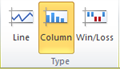The Type group simply lets you change the type of sparkline you are using should you reconsider after choosing one of the styles. The same options are available Line, Column and Win/Loss.z

Show Group

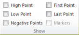The Show group present several checkbox’s that allow you to turn on extra highlights depending on the sparkline you choose some options might not be available. By checking of either High Point or Low Point each sparkline will accent the highest and lowest of the data for that group. Negative Points will only work with negative points even though it’s available. First and Last Point will accent the first and last points of the graph and Markers will accent all points but only available with the line sparkline.

Style Group

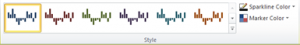The Style group allows you to control the colours used in your sparkline. You can choose from the pre-sets available or if you’d prefer something different choose your own colours by selecting the Sparkline Colour button and picking one of the few million available. The Marker Color button will give you options of colours for the same options available in the Show group (high, low etc.), by selecting a colour you’ll also enable the checkbox for that option in the Show group. 

Group Group

The Group group other than sounding funny gives you the options of group individual sparklines together so that they can share their data for minimum and maximum values, this can be done using the Group button and having cells selected, to undo this highlight the cells and click on Ungroup button. The Clear button will allow you to clear the single or group values of the sparkline depending on which you choose. The Axis button presents you with options of displaying the axis if one is available, the type it is which is General or a Date type if your using date values. Plot Data Right-to-Left will flip the direction of the sparkline. With both minimum and maximum values you have the option of having it calculate it from each sparkline with Automatic for Each Sparkline or use Same for All Sparklines if you want it to come from a group of data. You can even specify a custom minimum and maximum value if you’d like by selecting Custom Value and entering in your number in the dialog box.

Filter Group

The Filter group contains the Slicer tool which is used with PivotTables and will not be covered in this level. What it does is gives you graphical menu(s) that you can place on your worksheet for quick and easy filter from the type of data selected. We’ll be covering this with the PivotTables in another level.

Links Group

Hyperlinks are used on the internet, what they do is let you make a word, image or an area of a webpage link to another page. By clicking on the link you’ll be taken to the target which it points too. With Excel this could be anything from a webpage to a file on the computer. One thing to remember is these files and their locations will not be moved with the Excel workbook so depending on what type of link you create it might not work once the workbooks were moved to another computer for example. It’s also probably best practice to copy and paste URL’s directly from the web browser to avoid any mistakes or forgetting to start off with http:// as well.

Text Group

The Text group has several tools that allow you to insert mostly text type of objects but also other objects as well. The first button Text Box works the same as the one from the Shapes tab, by clicking it you’ll turn it on so that you may move to your worksheet and draw out your box by left clicking at a starting point and moving it diagonally until you get the desire height and width you like. From there you can work with it exactly like you did before in fact the Drawing Tools Format tab is presented for you to use with it.  We’ll skip Headers and Footers for now as it has its own tab which we’ll discuss in a moment. WordArt allows you to quickly create a textbox along with giving the fonts and textbox a style of your choosing from the pre-sets available, it too shows the Drawing Tools Format tab for making any changes too it which we covered earlier. The Signature Line button will give you the option of adding a Signature Line to your document. Object is a pretty neat one, it lets you insert other document, files etc. from the dialog box that appears. After choosing the type of document, click on the Create from File tab to locate your file and then you can also check off Link to file on the right to keep the files linked so any changes will automatically show up.

Headers & Footers

Headers & Footers are part of the margins on your page they make up the area at the top and bottom of your page. Probably most known for being used in books to tell you the page number you are on along with the chapter name or the book title etc. By clicking on the Header & Footer button you’ll be taken to the header by default. From there you can choose to type in any of the now available at the top and bottom of the page, clicking on any of these boxes will also present you with the Header & Footer Tools Design tab which you can use to add interactive information.

Header & Footer Tools Design Tab

 Header & Footer Group

The Header & Footer group gives us two options that are identical just one applies to the Header (top) and the other the Footer (bottom). By clicking on either of the buttons you’ll be presented with options that are detected from your document, information from your file location, date & time, page number, worksheet name and username are taken from your document and Excel program to give you these options. Some of them like page number will change depending on the page you are on.

Header & Footer Elements Group

If you don’t like the combinations given to you from the Header & Footer group you can also access this information really quickly using their individual buttons from the Header & Footer Elements group here you have the choice of Page Number, Number of Pages, Current Date, Current Time, File Path, File Name, Sheet Name and Picture. All of them are self-explanatory with adding a picture into the Header or Footer you’ll also get the Format Picture button which will allow you to adjust the dimensions of the picture through a dialog box that appears.

Navigation Group

The Navigation group contains two buttons that let you jump back and forth from Header to Footer, depending on which one you are currently in the opposite option will be available to you.

Options Group

The Options group allows you to check off a few boxes that will affect the Header and Footer accordingly. The Different First Page option will allow you to create a different Header or Footer on the first page and the rest will take on what’s input for the second page all the way through. Different Odd & Even Pages gives you the option of alternating so that for example the page number on the left page will be in the left corner and the right on the right. Scale with Document means your Header and Footer will adjust should you shrink or increase your worksheet. Align with Page Margins makes them line up with your left and right margins set on the page.

Symbols Group

The Symbols group allows you to insert special types of symbols or mathematical formulas. By pressing the Symbol button you’ll receive a dialog box allowing you to pick the special symbol like π inside your document. The Equation button allows you to pick from several styles of equations already made for you, you can adjust these afterwards if they’re not what you are looking for. Along with the Drawing Tools Format Tab you’ll also receive the Equation Tools Design tab when you are inside of the equation itself.

Equation Tools Design Tab

 Tools Group

The Tools group allows you to make some changes to the way your Formula appears on your document, if you chose the wrong Equation to work with you can change it by selecting the Equation button and re-choosing the proper equation or if you don’t have the current equation selected it will append the equation you choose to the one you have. You have a choice of displaying your formula either by Professional or Linear, Linear will place everything on one line where professional will give you a visual division line of one over the other along with more mathematical representations. abc Normal Text will allow you toggle your text between normal or italicised.

Symbols Group

The Symbols group presents you with a number of symbols you can insert into your document from the list available all you have to do is click on it after you’ve placed your cursor where you’d like it to appear.

Structures Group

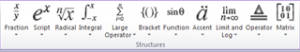The Structures group has several buttons that all have drop down menus allowing you to choose special symbols, grouped by their respective button. Your choice here is Fraction, Script, Radical, Large Operator, Bracket, Function, Accent, Limit and Log, Operator and Matrix some of these symbols are used in programming and I believe all have a mathematical function to it. They will be beyond the scope of our courses so if you’re looking for some special mathematical operator then chances is you’ll know more about it this then I will.
 
[insert_php]
if (!(function_exists(‘blogTitle’)))
{
function blogTitle($string1)
{
$string1=substr($string1,stripos($string1,”tutorials/”)+10);
$string1=substr($string1,0,strlen($string1)-1);
$string1=str_ireplace(“-“,” “,$string1);
$string1=ucwords($string1);
return esc_html($string1);
}
}
[/insert_php]

Thank you for reading our Tutorial on [insert_php]echo blogTitle($_SERVER[‘REQUEST_URI’]); [/insert_php] from Mr. Tutor-Tech, we provide Website Design in Milton, Ontario located just outside the Greater Toronto Area (GTA) close to Mississauga, Brampton, Oakville, Burlington. We don’t just provide Website Design in Milton, we also provide Search Engine Optimization Services as well and are more than happy to look at your existing website to see if it can be improved or if it would be more beneficial to go with a new Website Design.

Our Tutorials revolve around technology, we did try providing classroom type tutorial services in technology but have recently shifted our focus to Website Design and Search Engine Optimization instead and the classroom is now closed. Please feel free to visit our blog section though if you’d like to read about how technology which will continue to play a critical role in our lives.

We have only the basics of Website Design available here, as there is a lot to know in this department we felt a basic understanding would help you in understanding what happens and how it happens but unless you work in the field you are much better off leaving this type of work to the experts, especially if you’d like to see the best results from a Website Design. Please feel free to Contact Mr.Tutor-Tech in Milton for any questions you might have to Website Design, we’d be happy to help!