Microsoft Excel Level 4

Table of Contents

Formulas Tab

Insert Function Button

The Insert Function button allows you to quickly browse through a list of functions from the dialog box that appears after pressing it. It provides you with the ability of searching for a function using a keyword to search for or you can browse by category as well, making it easier to browse the almost 500 functions available. We’ll be listing some of these along with what they do. Functions are preprogramed calculations like the Sum function which adds up all the cells selected to give you a total. Like formulas functions begin with the = sign and usually take arguments to make them work. Arguments are information you pass to the function, depending on the function this can a range of cells, specific cells or other specific data. Within the Insert Function dialog box you’ll also get a description at the bottom of the function you have highlighted, chances are if you need a specific mathematical function that Excel already has it. Also using the dialog box to enter formulas will present you with a second dialog box, specific to the function you are entering. It will easily allow you to see the argument fields needed for the function and it will also give you a description of each of these fields as you click inside of them.

Function Library Group

AutoSum Button

Sum Function

The Sum function takes the data in the range you specify and adds it all up in the target cell.

Average Function

The Average function will add the selected range up and divide it by the number of cells with data in them, giving you the average of the selected area.

Count Numbers Function

The Count Numbers function is used to count the number of cells in the selected range.

Max Function

The Max function will return the highest value in the range selected.

Min Function

The Min function will return the lowest value in the range selected.

Recently Used Button

The Recently Used button will present the most recently used functions you’ve used in Excel and will change according to your usage.

Financial Button

The Financial button contains a number of functions used by financial institutions and unless you know exactly what they do can be confusing, we’ll be listing just a few here due to their complexity.

ACCRINT Function

The ACCRINT function will calculate the amount of interest returned on an investment that pays periodic interest. It takes 5 arguments, the issue date, first day of interest, the settlement date, rate of interest and par the principal amount.

ACCRINTM Function

ACCRINTM function is the same as ACCRINT function except it’s used when the investment is paid out in a final lump sum. Its argument list consists of the date of issue, settlement date, rate of interest, principle and basis which is the type of days of months and year are to be used 0 represents US 30/360 30 day months and 360 day years.

DB Function

Calculates the depreciation value of an item for the period of time using the fixed-declining balance method. It takes 4 mandatory fields and one 1 optional field for its options. The first field is the initial cost, next is the value at the end of its life, the length it’ll take to depreciate, the current term of depreciation and the optional month is for if you start using the product a certain time after purchase. Changing the current term will show you how much depreciation for that particular term.

FV Function

FV calculates the future value of an investment. It takes three mandatory arguments and two optional ones. The mandatory fields are the interest rate, the payment period and the payments made. If there is a principal investment this is entered in the Pv field and Type refers to payments made at the beginning or ending of the period.

PMT Function

Calculates the payments for a loan based on constant payments and interest rates. This takes 3 mandatory fields the interest rate, number of payments and the present value of the loan. The two optional ones are the Future Value of the loan if other than zero and type if payments are made at the beginning or end of the period, 0 the default is the end of the period and 1 is the beginning. 

Logical Button

Logical functions are used to compare data to see if the criteria are true or false, for example you could see if the value of cell c3 which has a value of 500 is greater than 100, which it is and would have the value True returned for the comparison.

AND Function

The first function listed in the Logical dropdown menu is AND, it takes two or more arguments and will compare them to see if they are all true in which case it will return true if any of them turn out to be false then false will be returned.

FALSE Function

False is actually not a function but a value that you can use in Excel to set a value to false for use in comparison, for example you could say if c3 with a value of 500 is less than 100 is equal to false then do something like make the field red for example because it’s not more than 100.

IF Function

The If function is used to do a logical comparison and can be set to do something if the result is true or if it’s false to do something else. Although the true and false fields are optional there’s no real use of the function otherwise, so you should be using one of these or just doing a logical comparison without the if then.

IFERROR Function

This function takes two arguments the value and what to do if there is an error in the value.

NOT Function

Not is used to return the opposite of value or comparison, so if you were to enter the value of not(true) the result would be false and vice versa.

OR Function

The Or function like the And function compares two or more pieces of data except if anyone of these values is true then true will be returned otherwise it’ll return false.

TRUE Function

True is the same as False and not a function but a value that you can use in Excel to set a value to true for use in comparison, for example you could use if c3 with the value of 500 is less than 100 is equal to true then do something like make the field green because it’s a good value. 

Text Button

BAHTTEXT Function

With computers text characters are associated with a number known sometimes you’ll have to work with them in this format which makes it hard to read, this function will convert the number to a character.

CLEAN Function

Clean removes any nonprintable characters from your data.

CONCATENATE Function

Concatenate combines text together, you could use it for example to take field 1 which is first name and field 2 which is last name to combine them together in field 3 which is full name.

EXACT Function

Exact compares two strings to see if they are identical, this comes in handy when comparing something like a logged in user to one in the spreadsheet or something like that.

FIND Function

The Find function takes two mandatory arguments the String of text to search and the text to search for and an optional field where you enter the starting point of the text being searched. For example you could use = find(“This is my place”,”place”) to find out if the word place exists in the sentence, if it does the function will return the first character number of where the found text starts.

FIXED Function

You can use fixed to round number to a certain decimal point and to include comas or not.

LEFT Function

This will return the text starting from the left side to the amount of characters you specify and to be used properly takes two arguments the text and the last character where it cuts off at.

LEN Function

Len takes one argument a string and returns the length of that string.

LOWER Function

Lower will return all the characters in a string in lower case.

MID Function

MID works just like the left function except it takes an additional parameter and that’s the starting point of the string, for example =mid(“george’s text”,9,4) would return the word text.

PROPER Function

Converts text to proper case with the beginning of each word captialized.

REPLACE Function

You use this function to replace text inside of a string, it takes three arguments the original string, the text to search for and the text to replace it with.

REPT Function

Will take the string you enter and repeat it a certain number of times.

RIGHT Function

Right works exactly like Left except in the opposite direction and will start off from the right side of a string.

SEARCH Function

Search works exactly like Find the only difference is that Find is case-sensitive and Search is not.

T Function

You use the T function to examine data to see if it’s text or not.

TRIM Function

Use the Trim function to remove extra spaces from a field these can be trailing spaces or even double spaces between words, it will leave single spaces found between words.

UPPER Function

You use the Upper function to transform text value to uppercase.

VALUE Function

You use this function when a numerical value is being returned as text and you would like Excel to treat it as a number instead. If field c3 had “George made $5” then you could use multiple functions like =right(c3,1) which would return the value of 5 as a text because of the original content, to convert this you would wrap the right function inside of value and now the return value would be a numerical value capable of comparison to other numbers, the final formula would look like =value(right(c3,1)).

Date & Time Button

Pressing this button will present you with a dropdown menu that has all the functions which revolve around dates and times which are treated a differently in Excel from other text and numbers.

DATE Function

Date function will convert the value passed as an argument to a properly formatted Excel date type or serial number.

DATEVALUE Function

This will convert the argument to a date value serial number. Computers can treat days differently depending on how they were setup that’s why Excel also works with date serial numbers which is a number increasing by 1 for each day starting at January 1 1900, so Aug 22 2008 would equal 39682. 

DAY Function

The Day function will take it’s date argument and extract a day from 1-31 of that month from it.

DAYS360 Function

Days360 calculates the difference between two dates based on 360 day calendar, it takes two arguments the start date and end date.

EDATE Function

The Edate function is used to add/subtract month(s) from the initial calendar date, it takes two arguments. The first one is the original date and the second is the interval in months, placing a 1 here will add a month to the original date a -1 will subtract a month from the original date.

EOMONTH Function

This function works the same as Edate except it return the last day of the month instead of the same day of month.

HOUR Function

The Hour function return the hour portion of a time in military format ranging from 0 to 23.

MINUTE Function

The Minute function returns the minute portion of a time ranging from 0 to 59

MONTH Function

The Month function returns a numerical value from 1-12 for the month portion of  date field.

NETWORKDAYS Function

The Networkdays function returns the number of work days between a start date and end date which are the two mandatory arguments this function takes. It also lets you enter holidays in with its third optional parameter.

NETWORKDAYS.INTL Function

If you find yourself needing to calculate workdays where the weekends fall on different days for the employee then you would use the NETWORKDAYS.INTL function, which allows you to specify the days that are weekends in a 4 parameter.

NOW Function

The NOW function takes no arguments and will bring back the current date or date serial depending on the field formatting.

SECOND Function

The SECOND function returns the seconds from a time.

TIME Function

The TIME function will take a time value and return a percentage of that time relative to the day, so it ranges from 0 to 0.99999999 which is from midnight to 11:59:59 PM.

TIMEVALUE Function

The TIMEVALUE function is exactly the same as the TIME function except that it will accept a string representing time as a value.

TODAY Function

The TODAY function will return the current date in a date format or serial format depending on the cell formatting.

WEEKDAY Function

The WEEKDAY function will return a numerical representation of the day, 1 for Sunday to 7 for Saturday.

WEEKNUM Function

The WEEKNUM function will return the number of the week the value falls on.

WORKDAY Function

The WORKDAY function will take a start date and a number of workdays and find the end date skipping weekends. It can also be used with a negative number to work its way backwards. A third optional argument is there for holidays.

WORKDAY.INTL Function

Works in the same way as WORKDAY except you can specify with a 4^th argument when the weekends fall for employees that might work on Saturday and Sunday kind of thing.

YEAR Function

The YEAR function returns the year from a date value.

YEARFRAC Function

The YEARFRAC function will return a percentage of where the end date falls from a yearly calendar with a start date specified. This is an easy way of calculating how much of a year an employee has worked for something like benefits for example. It also takes a third argument a number from 0 to 4 which represents the Day Count Basis by default it does a 30 day month and 360 year. 

Lookup & Reference Button

This button will offer you a dropdown menu with a number of options that will lookup or reference information from the same worksheet other worksheets and even other workbooks. We’ll only be discussing two of the functions here which work much in the same way just one is vertical and the other horizontal and they are the VLOOKUP and HLOOKUP functions

HLOOKUP & VLOOKUP Functions

What these functions do is allow you to create a field where you type in a search criteria, you give it the table or area to search and then you tell it what piece of information you’re looking for, for example price which will be returned in the field you enter the formula in. There’s one last bit of criteria for this function and that’s do you want to find an exact match or a close one. This depends on what you’re using it for, in our example above where we search for a product we want an exact match but if you were looking for something that had percentages between certain ranges of numbers then you’d probably look for something close. To tell Excel an exact match is need the value entered is false and for close is true by default Excel will look for something close to the search criteria. In the following picture you’ll see an example of the VLOOKUP in use, (1) shows you the formula used for this VLOOKUP which resides in the selected box of F3(3). It looks up the first criteria from the formula in F1(2) from Table1(4) which is the second argument of the formula. The third argument of the formula is the number of the column that contains the value to return, from our range our table we always count from the left to the right so products is our first column, description the second and price the one we need the third which is entered into the third argument of the VLOOKUP function. The last argument is set to FALSE meaning we want an exact match.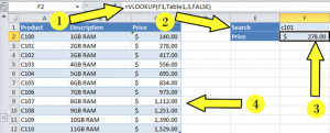

Math & Trig Button

The Math & Trig button will give you a long list of functions associated with various mathematical formulas, if you’re a rocket scientist or physicist then you might use these quite a bit otherwise if you’re searching for some special function like square root or the power of which you use on a calculator then this is where you’ll find those functions as well.

More Functions Button

The More Functions button couldn’t be more self-explanatory if they tried, it’s more functions available broken up into a few groups to help you search for them they are Statistical, Engineering, Cube, Information and Compatibility. Excel has close to 500 different functions all of which are available through the Insert Function Dialog box but these buttons covered here contain most of them and after using them you’ll quickly navigate through the different groups to find the one’s you’re looking for. Another thing to keep in mind is that if you find yourself using a particular function a lot you can add it the quick access bar.

Defined Names Group

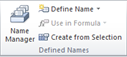When you get used to working with Named Ranges then this group will make it easy for you to find, identify, edit and remove them from your workbook. The first button here Name Manager will present you with another dialog box that will show you all the named ranges in the workbook. From this dialog box you can edit, add or even delete named ranges but there are much easier ways of adding them. You can also filter ranges here if working with a longer list. The Define Name dropdown menu will either let you name the selection or to name it from existing range name. When writing formulas you can enter range names into them from the dropdown list here presenting you with all the ranges available in your workbook. The last button here Create from Selection allows you to select an area which includes the range name in it, then in the dialog box you tell Excel where the names for the range are by selecting top, bottom, left or right combinations.

Formula Auditing Group

The Formula Auditing group presents with several useful tools for troubleshooting your worksheet for errors. The first two buttons Trace Precedents and Trace Dependents will present arrows that will show you what cells depend on that formula (Precedents) or what formulas depend on the cell (Dependents). By clicking it multiple times it will branch out each time expanding the function another level until the highest level is reached. This could be very useful say when copying over data and a cell points to an absolute reference that’s moved or vice versa, by clicking on one of the two functions you’d quickly identify that the cell needed might be empty or has the wrong information etc. The arrows can easily be removed when done viewing by clicking the Remove Arrows button, which with the dropdown menu can be used to remove specific types of arrows. The Show Formulas button will make the cells display the formula inside of them instead of the result from the formula and is used as a toggle switch to go back and forth between views. In the example on the next page (1) is tracing the precedents from cell F2 this show’s two arrows heading into this cell one from F1 and the other from A2, if clicked again it would show C2 to C12 as well but that would have made it harder to see the trace of Dependents (2) arrow coming from C12 pointing to F2. You’ll also notice that the cells are displaying their formulas instead of values as you can see in column C and in cell F2, this is from the Show Formulas toggle.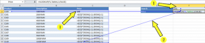

Using the Error Checking button you’ll have Excel check your worksheet for errors or what it thinks might be mistakes because something doesn’t conform to the rest of the cells around it. By clicking on the arrow you’ll also have the option to Trace Error, slightly changing the example from above I’ve created an error on the worksheet and used the Trace Error function which will now display an arrow pointing to the offending cell.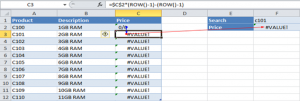

The Evaluate Formula button will present you with a dialog box that will display your formula inside of it and is a useful way of troubleshooting long complex formulas with multiple steps in them. This dialog box by clicking Evaluate will take you through the steps 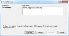that Excel uses to come to the final result. As you move through the different stages of the equation Excel might detect other cells that contain a formula as well, in this case you can use the Step In button to see it’s formula as well, when you’re done simply click Step Out to return to the Evaluate process.

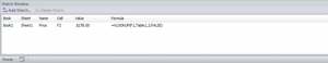The last button on the Formula Auditing group is the Watch Window which presents you with a new window which you can dock or undock to the Excel window whichever you prefer. With this window you have the option of adding cells to its list of items to watch. This information will present you with the book name, sheet name, range name, cell location, value of the cell and the formula of the cell for you to monitor as you make changes to your worksheet.

 Calculation Group

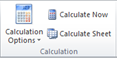Excel by default will automatically recalculate anything as soon as a change is made inside the workbook. This typically works great but if you’re using a lot of data and over a network this could slow down quite a bit, causing frustration as you have to wait for Excel to finish doing its thing.  To get around this problem you have the option of setting these settings to Automatic (default), Automatic Except for Data Tables or Manual. By setting this to Manual you can use the Calculate Now and Calculate Sheet buttons to recalculate. Calculate Sheet will recalculate the current worksheet where Calculate Now will do the whole workbook.
 
[insert_php]
if (!(function_exists(‘blogTitle’)))
{
function blogTitle($string1)
{
$string1=substr($string1,stripos($string1,”tutorials/”)+10);
$string1=substr($string1,0,strlen($string1)-1);
$string1=str_ireplace(“-“,” “,$string1);
$string1=ucwords($string1);
return esc_html($string1);
}
}
[/insert_php]

Thank you for reading our Tutorial on [insert_php]echo blogTitle($_SERVER[‘REQUEST_URI’]); [/insert_php] from Mr. Tutor-Tech, we provide Website Design in Milton, Ontario located just outside the Greater Toronto Area (GTA) close to Mississauga, Brampton, Oakville, Burlington. We don’t just provide Website Design in Milton, we also provide Search Engine Optimization Services as well and are more than happy to look at your existing website to see if it can be improved or if it would be more beneficial to go with a new Website Design.

Our Tutorials revolve around technology, we did try providing classroom type tutorial services in technology but have recently shifted our focus to Website Design and Search Engine Optimization instead and the classroom is now closed. Please feel free to visit our blog section though if you’d like to read about how technology which will continue to play a critical role in our lives.

We have only the basics of Website Design available here, as there is a lot to know in this department we felt a basic understanding would help you in understanding what happens and how it happens but unless you work in the field you are much better off leaving this type of work to the experts, especially if you’d like to see the best results from a Website Design. Please feel free to Contact Mr.Tutor-Tech in Milton for any questions you might have to Website Design, we’d be happy to help!