Microsoft Excel Level 5

Table of Contents

Data Tab

Get External Data Group

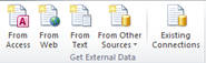The Get External Data group allows you to import data from different sources depending on which button you choose. Your options here are From Access which will retrieve information from an Access Database. The next option is From Web which allows you to enter a URL and in a type of web browser, once you are the page or site you’d like to import from you can simply click Import to grab everything or anywhere there is a table inside this browser will have an arrow beside it, you can click on this to grab this table and it will change to a checkbox when you have. The From Text button will allow you to import from a text document such as Word, Wordpad and Notepad etc. From Other Sources gives you a dropdown menu that will give you a few more options for importing data and they include From SQL Server, From Analysis Services, From XML Data Import, From Data Connection Wizard and From Microsoft Query. Typically importing a file is pretty simple but depending on the file type there might be options or settings you’ll need to adjust to make this happen or at least properly. If you’re bringing the data in from something other than a file or the internet then you’ll need to know where to find the file or how to setup a connection to your database in order to retrieve it, this will be outside the scope of this course. The last button Existing Connections displays all the connections available to your workbook, if you have made any that is. It also has three connections setup that you can use to retrieve information on currency, stocks and major indices, just click on the connection you’d like then if prompted for a location specify where you’d like to drop the information in your worksheet.

Connections Group

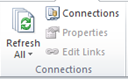The Connections group allows you to work with your connections and settings. The first button will allow you to refresh all if pressed or provide you with a dropdown menu if the arrow is clicked. Here you have the option of Refresh All, Refresh which will do the connection selected, Refresh Status will give you the update on the process and Cancel Refresh will stop it. The Connections Button will show you all the active connections to your workbook. From here you can also delete, add new ones or even refresh them as well. The Properties button will present you with another dialog box which will give you a number of options in regards to your connection. Here you can name your connection, give a description and enable other settings. The Refresh control area allows you to set how you’d like the connection to refresh, like when opening the file or every so many minutes and removing the data before saving. Under the definitions tab you control the location of the connection file along with the connection string and more settings which you’ll need to know ahead of time to make a connection.

Sort & Filter Group

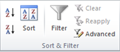The Sort & Filter group starts off with two buttons to quickly sort selected data in Ascending or Descending order. The second button the Sort button works just like the one of the Home tab and presents you with a dialog box where you can enter multiple sorting criteria. If you find yourself wanting to filter data but not wanting to create a table then the Filter button is what you want. By selecting the data you’d like to Filter and then pressing the Filter button you’ll be presented with a few options, here you’ll need a heading as the top row will be omitted from the filtering and an arrow like the one in available in Tables will be available, it will also function in exactly the same manner as we discussed in a previous level. You can also Clear or Reapply these filters once they’ve been used. The Advanced filtering button will give you a dialog box asking you where your information is along with where your criteria is, which we’ll explain in a second just note that you have two other options here a check box at the bottom Unique records only which will remove duplicates and a radio button at the top where you can Filter the list, in-place or Copy to another location which will open up the Copy to field and allow you to specify the location. With the Advanced filtering you’ll need to create a second table on your worksheet that has the same headings as the table you’d like to filter from. You don’t need to copy all the headers just the ones you plan on filtering. Once you’ve done that you can enter information underneath the header and anything along that row will be put together with an and clause between them meaning all the criteria is to be met, in order to do an or clause you need to move down a row for each or. An simple example of the Advanced filter is below where we created a second table just above and gave it the <500 value in the price tag, this means return anything under $500 which was in the table right beside it using the Copy to another location option. Here our main table including the headers is the List range and our Search Criteria table including the headers is the Search Criteria, it’s very important that the fields used for filtering are named exactly the same and selected.  In our example below (1) is the criteria table, (3) the information table and (2) is the results copied over from our filter using that option.

Data Tools Group

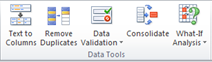The Data Tools group has a few nifty tools in it, the first one is Text to Columns which will take a column of information say first name and last name together, then split it apart to have two separate columns that would be first name and last name separately. To use this tool the first thing you need to do is select the data you’d like to adjust. Once that’s done click on the button to get the dialog box which will ask you a series of questions before proceeding with the operation. It’s also a good idea to insert a new column beside the one you’ll be using the function on as the data will enter this column unless you specify one somewhere else or at the end of a table as the destination point. There is a little bit of knowledge you’ll need before 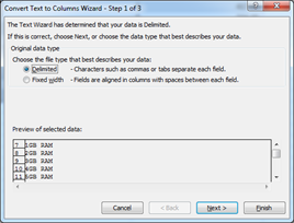splitting up this column, the first question from the dialog box is if this is Delimited or Fixed width. Your choice depends on how your data is formatted, Delimited means that there is some common character separating the words and fixed width is more of the last name starts so many characters after the first name which will always remain the same. The next question depends on the answer to the first if it was Fixed width then you’ll receive a dialog box asking you for the character point where the last name starts. With Delimited you’ll be asked what special characters separate your words, is it a tab, semicolon, comma, space or other which you can specify. The last of the series of questions is about where you’d like to put the info by default it will start where it is but you can place it somewhere else with the Destination box, you also tell Excel what kind of data you’d like it to be here is it general, text, date or just skip the format altogether. Advanced will give you more options on numerical formatting. Both the second question and the last question will give you a preview of what your data will look like, the last thing to do is click Finish.

The Remove Duplicates button will take away any duplicate pieces of information from the area you select. After selecting the data click on the button to receive a dialog box which will ask you what columns you’d like to check. If you have multiple columns then they will have to have the same information in all the columns you select to be considered a duplicate. AS our dialog box here displays three rows Product, Description and Price. Leaving the items checked this way would mean all three columns need to have the same information in more than one row to be considered a duplicate. If for some reason I had a different description but the same product number this wouldn’t work, so instead I would just check off Product and this would do the trick then.

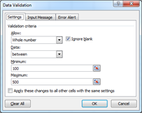
With Data Validation you can tell Excel that you’d like to use a certain type of data for that cell and give it criteria as well. This will prevent anyone entering invalid data, you can also specify a drop list from which to choose data from here as well. In our example here, we set cell C10 to a number value only and it has to be between 100 and 500 which it wasn’t prior to us giving this setting. If we tried entering the value after it was set we would get a prompt saying we can’t. From the dropdown list of the Data Validation button you have the option of Circle Invalid Data to highlight data that doesn’t meet the requirements like in our example, to remove these circles simply click Clear Validation Circles.

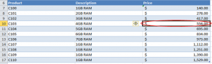
When you are working with multiple sheets that contain the same type of data, like say monthly reports.  You can use the Consolidate button to put them altogether at the end of the year in a yearly report. The beauty is that the columns don’t have to be in the same order or the same columns have to be in each worksheet as Excel can gather this from the header information as long as 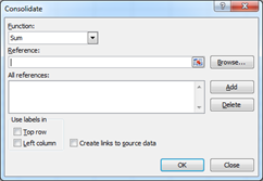the appropriate columns are named the same everything will work out. After pressing the button you’ll receive a dialog box asking you for some information. The first question is the Function or operation you’d like to perform on the data, by default its Sum which will add the information up in a total type summary. The next box Reference is your selection of the data, once you’ve done this you click the Add button to add it to the list, you do this for as many worksheets as you’d like to consolidate and can use the Delete button to remove any should you change your mind or make a mistake, remember to choose the header information if it’s there. The next two decisions you’ll need to make is to let Excel know where the header information is Top row and/or Left Column. If you’d like this report to get updated from its source information then click Create links to source data. Once you’re done click OK and you’ll have a consolidated worksheet.

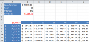
We’ll be using the picture above while we talk about the What If Analysis which gives us three options from the dropdown menu. The first one is Scenario Manager which will present you with a 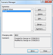dialog box, asking a few questions. In this box we Add different scenarios by clicking the Add button you’ll be asked for a Scenario name and Changing cells in another dialog box. You can name the scenario anything you’d like as well as give it a description which means something, this does not affect the results. The Changing cells box is the main concern here and this is where we highlight the cells we’ll be working with and changing. Using our top table we could reference cell B3 here so that we could play with different interest rates, after selecting this cell and pressing OK, we’ll be asked for the new information we would like to set this box to. It’s a good practice to create an original values scenario for your first one so that you can easily reset the information. You can repeat this scenario as many times as you’d like, so we could add a bunch of new one’s that contain the following percentages 5.1{463c70c279fb908728b910a090d44fbe4ae7aabcd875de9c1a518a8c8e2be8bd},5.2{463c70c279fb908728b910a090d44fbe4ae7aabcd875de9c1a518a8c8e2be8bd},5.3{463c70c279fb908728b910a090d44fbe4ae7aabcd875de9c1a518a8c8e2be8bd} and 5.4{463c70c279fb908728b910a090d44fbe4ae7aabcd875de9c1a518a8c8e2be8bd}. Once we’ve entered these values in different scenarios we can use the main dialog box to shift between the different scenarios by either double clicking on them or by selecting the proper one then clicking show. As you change between the different scenarios Excel will recalculate the result allowing you to see the different type of payments.

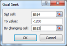The next option from the What If Analysis is the Goal Seek, here we could use this function with the top table to find out what interest rate we can afford if we could afford a maximum of say $1200 for monthly payments. The key to this function is that there must be a formula in use out of the selection in order for it to be able to perform reverse calculations. We used the PMT function in our top table to calculate the payments. Using the Goal Seek dialog box pictured here we entered the cell B4 as the cell we know the value we know, with the value being -1200(negative for payment) and the changing cell is B3, after clicking OK the cell B3 changes to 6{463c70c279fb908728b910a090d44fbe4ae7aabcd875de9c1a518a8c8e2be8bd}, we get a second dialog box where we can confirm the changes by clicking OK or Cancel to avoid making the changes.

The last function of the What If Analysis is Data Table and is being displayed as the second table in our picture at the top of the previous page. You’ll notice in the corner A7 of our table we copied 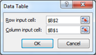the same formula from B4, the second thing we did was add payment terms horizontally and different loan amounts vertically, Excel actually filled in the rest of the data in a snap of a finger.  After we created our table just described, we need to select everything in it from the formula down to the last term and the last loan amount. We can then click on the What If Analysis button and click on Data Table to receive its dialog box. Since we’ve already selected our table Excel know that we’ll be working with that area, the only thing we need to do now is let Excel know what values are running vertically and horizontally. As you’ll see in the dialog box picture we set these to B2 which is our term for the horizontal row which is 10, 20, 30, 40, 50 and 60. We set vertical column to B1 which is our loan amount and was filled out in the table with the amounts of $15,000, $16,000, $17,000, $18,000, $19,000 and $20,000. After clicking OK you’ll see Excel fill in the rest of the information like in our picture above.

Outline Group

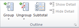
The Outline group allows you to group pieces of data together that way you can collapse it and temporarily hide it to make looking at other piece of information 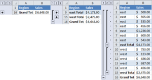easier, typically groupings will present other information when hidden a perfect example would be a list of items purchased and then the total at the bottom. What you could do is group all the items purchased together that way when they’re collapsed all you’ll see is the total of all the items. By highlighting the data you’d like to group and pressing the Group button will achieve this, the Ungroup button will remove the grouping from the selected cells. Subtotal will group items for you along with combining like items together and running a sub-total for each of them and a grand total will be at the end. Just like I mentioned a second ago you can shrink levels and see just the sub-totals leading into the grand total instead of looking at every single item. Show Detail and Hide Detail will expand or collapse the groupings which can also be done using the + and – signs that’ll be available beside or on top of the column or row header information as seen in the picture, which are also represented in the corner by numbers. By clicking on 1 you’ll collapse all levels and display the minimum amount of data and as you go up each number another level will open up for you. In our picture going from left to right we move from completely collapsed showing only grand total to completely expanded showing all items and the middle just the sub-totals.

View Tab

Workbook Views Group

The Workbook Views group allows you to change between different views with its first three buttons. Normal is the default view you have when you open up Excel, you can change between Page Layout view and Page Break Preview which will let you see what the page looks like when it would be printed or to easily set page breaks for printing. The Custom Views button allows you to save the current view as a pre-set so that you can jump between your favourite views without having to repeat all the settings involved, this includes the zoom level along with where in the document you are and other features like frozen panes which we’ll discuss shortly. Full Screen will take away the ribbon and everything else expanding your worksheet across the whole monitor from top to bottom and left to right.

Show Group

The Show group has a few checkboxes for us to turn on/off which will show or hide that particular Excel object. The first one Ruler maybe greyed out depending on the current view you are in, it’s only available with the Page Layout view and by checking it off means it will be displayed and removing it will hide it. Gridlines are the squares around each cell that you see while working on your document they can be printed if so desired but not by default, it’s there mainly to make working easier but if found annoying can be hidden by removing the checkbox. The Formula Bar although a huge necessity when working with Excel can also be hidden by removing its checkbox. The last item of this group is the Headings checkbox which will hide the row and column headings in Excel this is are where excel displays A, B, C, D, E etc. for columns and 1, 2, 3, 4, 5 etc. for the rows, by removing this checkbox you’ll no longer see these.

Zoom Group

The Zoom group controls the zoom of your object, with the Zoom button you’ll receive a dialog box with several options from typical zoom settings along with a custom option where you can specify the zoom level in a percentage. Two of these options are available as other buttons on the Zoom group and they are 100{463c70c279fb908728b910a090d44fbe4ae7aabcd875de9c1a518a8c8e2be8bd} and Zoom to Selection. The 100{463c70c279fb908728b910a090d44fbe4ae7aabcd875de9c1a518a8c8e2be8bd} button will zoom in or out to the 100{463c70c279fb908728b910a090d44fbe4ae7aabcd875de9c1a518a8c8e2be8bd} mark which is the default for Excel. By selecting Zoom to Selection Excel will zoom in as close as possible to make your selection fit across the window. 

Window Group

While working in Excel you might find yourself using multiple workbooks which are opened in new windows. This group allows you to control how you’d like to view these windows along with opening new ones and switching between them. The first button from this group is the New Window button and by clicking it will open a new workbook. The second option Arrange All will give you a dialog box offering you options on how you’d like to view your windows, these are Tiled, Horizontal, Vertical and Cascade.  The Freeze Panes button will give you an option of freezing certain cells so that they don’t move with the scrolling of the window. Your options here are to Freeze Panes which will freeze cells both vertically and horizontally to where you current active cell is. The other two options here Freeze Top Row and Freeze First Column will either keep the top row or the first row frozen depending on your choice. These functions are mainly useful in keeping your header information in sight while you scroll so you can easily see that the bottom of the column you are looking at for example is in the Price field. When there are frozen panes on your sheet this is also the button you click to unfreeze them and this option will become available to you at that time. The Split button allows you to create breaks in your worksheet giving you two or more windows inside of one and each one can be scrolled separately unlike the frozen panes, it also acts as a toggle button so by clicking it again you’ll remove the splits. Using the Hide and Unhide buttons you can hide the current worksheet or unhide hidden worksheets which will be displayed in a list inside of dialog box after pressing Unhide. When working with two windows that you’d like to compare against each other you can use the View Side by Side button which will display both windows inside of one, by default the Synchronous Scrolling toggle button will be enabled. What this means is when scrolling in one window the other will scroll in exactly the same way. You can disable this and keep this view by clicking the Synchronous Scrolling button again. While it’s enabled should the two windows become out of sync then you can press the Reset Window Position button to reset them to the same point. You might find yourself working with certain multiple workbooks a lot, instead of having to open each one and then lay them out to the view you like each time you can save this, using the Save Workspace button which will save your file as an .xlw file. By opening this file all the workbooks and the view you had will be restored. The last button of this group presents a dropdown menu and when more than one workbook is open will display each one that is for you to easily jump between. 

Macros Group

Macros is a nifty way of recording steps you take in your worksheet, so that you may play them back and repeat the steps as much as you’d like saving you time from performing these steps over and over again. It’s fairly straight forward to use but to modify not so easy, you’ll need to know VBA programming to modify it. VBA is out of the scope of this level so if you 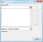need to make changes to a macro you’re better of re-recording it. It’s best to have everything ready along with knowing what steps you’ll be taking before recording the macro. Once you’re ready simply click on the  button which will give you the dialog box where you can view existing ones or add new ones. You can also click on the Record Macro option from the dropdown menu if you click the arrow. One other thing to keep in mind when using Macros and that’s will you be using it from the exact same spot each time or will the active cell dictate how t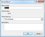he Macro responds. If you want the Macro to perform the same steps at different locations then you’ll need to enable Use Relative References from the dropdown menu before proceeding. The View Macros option is just like clicking on the Macros button and will present a dialog box where you can run or delete Macros, along with Edit which as explained requires VBA knowledge. The Record Macro dialog box asks you a few simple piece of information before you start recording and that’s the Macros name, where you’d like to store it and a description. One other item here is a shortcut key which you can use to run the Macro instead of having to go through view Macros and then selecting it and running it from the dialog box. Once you hit OK here you’ll be recording everything you do, which will get replayed when you run the Macro as well so be careful. After you perform all the steps you’d like the Macro to record you’ll need to stop it, this is done through the dropdown menu from the Macro button, where the Record Macro option used to be.
 
[insert_php]
if (!(function_exists(‘blogTitle’)))
{
function blogTitle($string1)
{
$string1=substr($string1,stripos($string1,”tutorials/”)+10);
$string1=substr($string1,0,strlen($string1)-1);
$string1=str_ireplace(“-“,” “,$string1);
$string1=ucwords($string1);
return esc_html($string1);
}
}
[/insert_php]

Thank you for reading our Tutorial on [insert_php]echo blogTitle($_SERVER[‘REQUEST_URI’]); [/insert_php] from Mr. Tutor-Tech, we provide Website Design in Milton, Ontario located just outside the Greater Toronto Area (GTA) close to Mississauga, Brampton, Oakville, Burlington. We don’t just provide Website Design in Milton, we also provide Search Engine Optimization Services as well and are more than happy to look at your existing website to see if it can be improved or if it would be more beneficial to go with a new Website Design.

Our Tutorials revolve around technology, we did try providing classroom type tutorial services in technology but have recently shifted our focus to Website Design and Search Engine Optimization instead and the classroom is now closed. Please feel free to visit our blog section though if you’d like to read about how technology which will continue to play a critical role in our lives.

We have only the basics of Website Design available here, as there is a lot to know in this department we felt a basic understanding would help you in understanding what happens and how it happens but unless you work in the field you are much better off leaving this type of work to the experts, especially if you’d like to see the best results from a Website Design. Please feel free to Contact Mr.Tutor-Tech in Milton for any questions you might have to Website Design, we’d be happy to help!