
PivotTable Tools Options Tab. 5
PivotTable Group. 5
Active Field Group. 5
Group Group. 6
Sort & Filter Group. 6
Slicer Tools Tab. 6
Slicer Group. 6
Slicer Styles Group. 6
Arrange Group. 7
Buttons Group& Size Group. 7
Data Group. 7
Actions Group. 7
Calculations Group. 7
Tools Group. 8
Show Group. 8
PivotTable Tools Design Tab. 8
Layout Group. 8
PivotTable Style Options Group. 9
PivotTable Styles Group. 9
PivotTable Trick. 9
PivotTables

PivotTables are a great tool for gathering data and grouping it together in some meaningful manner for analysis. The beauty is you can adjust or create different reports easily and just shift it on the fly to see the information in a variety of ways. You can also build Pivot Charts from this data and have it adjust automatically as well. We’ll discuss charts a bit after we conquer the tables first, but I wouldn’t be too afraid as far as the charts go it’s exactly the same as you’re used to with the regular charts they just bring the Pivot functionality to them and once you understand the tables you won’t have any problems with charts.
 PivotTables work best with one row of header information, this would be something like a phone book with name, address, phone no etc. per row or like in our example a list of employees with their salaries, positions, departments and start dates. These can be used to group the information together in some other meaningful manner, like a summary of average salaries per group, {463c70c279fb908728b910a090d44fbe4ae7aabcd875de9c1a518a8c8e2be8bd} of total salaries per position. How many people started and the list goes on not to mention there’s filtering as well. Information like Forbes list of the richest men in the world and their net worth from 2010-2012 can be used Excel will shove whatever data you give it into the PivotTable but the only thing is there’s nothing to group information, the names are already
 unique fields and the years are already totaled up, that doesn’t mean you can’t group information by a certain range of net worth, grouping it by last name to combine family’s. So again it’s not to say you can’t use this information in PivotTables it might just become difficult to group information in some meaningful way. When working with PivotTables it’s also nice to use data from a data table, you can use just data in a range if you’d like but when referencing a table you reference the name so if you add information the PivotTable will be able to use it by refreshing the data first. Otherwise it’ll point only to the ranges you specified and not the new ones you add after.
To Insert a PivotTable you’ll first want to either be inside the table you’d like to use or with the data information highlighted,  then move to the Insert tab and press the PivotTable button, you can choose here also to make a chart at the same time but the table will vary somewhat with that
  direction and you might not have the information you’d like to view available because of it, I recommend building a table first and then a chart after from the table. It’s also not necessary to have the data selected if it’s in a range you can specify it later but it’ll save you a step if you do. Once you receive the dialog box you can specify the range or reference to the table if you didn’t have the data selected. Here you also have the option of telling Excel where
  you’d like to put the PivotTable. In our example above you’ll notice that it says Table 1 for the Table/Range, this will ensure new data will make its way into the PivotChart when you press the Refresh button on its tab which we’ll talk about shortly. Once you’ve pressed OK you’ll see a new worksheet open up because of our choice in the dialog box. On it you’ll see the PivotTable image on your left hand side and the PivotTable field list on the right. There are a few ways to have the pivotTable display stuff, you ‘ll notice at the top of the pane you have the header information from our table, by checking these off Excel will take a guess at where on the PivotTable they should go. This usually work from the data contained. As you check them off you’ll notice them appear in one of the four boxes below which are Report Filter, Column Labels, Row Labels and Values. Column and Row Labels are self explenatory that’s where the header displayed in there will display its information. The Report Filter is used to not display this information to be able to use it to filter information being brought back, on it’s criteria. The Values area will perform calculations on the groupings which you’ll be familiar with once you see them. By clicking and holding down the left mouse button over the header information you can also drag it to the box you’d like it to be in and before checking it off you can the same from the top window as well. With a few extra steps you’ll end with a table like the one you see here.
PivotTable Tools Options Tab
After you’ve created your PivotTable you’ll have two new tabs available to you the first one is the PivotTable Tools Options tab, the other one is the Design tab.
PivotTable Group
 The textbox at the top of the PivotTable group is where you give your tale a more meaningful name if you’d like. The Options button will bring up a dialog box where you can control several settings for the way the PivotTable behaves, typically the default settings are just fine but if you’re looking to fine tune something or change certain behaviour of the PivotTable then check here first. Most of its self-explanatory when looking at the description but you can always use the help ? in the top right corner.
Active Field Group
 The Active Field group will display what field you are currently in inside your talbe in the text box in the top left, as you move around your table this will change
  according to what field is driving the information. The Field Settings button will also display a different dialog box depending on what field you are in and what type of roll that field is playing. If it’s not a calculated field then you have the opportunity to convert it to one here. Typically this is used to change the function of the calculation being performed on a particular field. Excel typically will use the Sum function to add the totals up, you’re free to change that using the dialog box, you can also display the way the information is being presented say for example you do use the sum function to add up the totals, you can choose to display them as percentages of the grand total, this way you can see what percentage is the highest for profits for example. If you are in a collapsible field then you’ll be able to do so either by the +/- signs by the field which could be hidden with an option so a secondary option is available to Expand or Collapse Entire Fields.
Group Group
 Here we can combine items together to combine their calculations for example. Say you have North-East, North-West, South-East and South-West divisions you could group the North and South together to combine their information for a certain type of presentation. The Group Field button will allow you to group the active field in different manners for example if you were in a date field you could group these together by the year, year & month, weekly and many other ways including ones for numbers and text fields.
Sort & Filter Group
 The Sort and Filter group works just like it does with a regular table or selection. Except there are two shortcut buttons for sorting the active field either ascending or descending
  depending on your choice. The Insert Slicer button is the same as the one available on the Insert tab, what it does is allow you to select which headers you’d like to work with through a dialog box, by checking off the headers and then pressing the OK button a window for each header will be displayed, in here you’ll see a list of the grouped fields for that header. Depending on current filtering they will either all be highlighted or just the ones bringing back information will. You can use these boxes to filter information from your table now, the bonus is you’ll be able to visually see what information is being filtered. At the top right you’ll notice the remove filter button which will clear the current filter and make all the fields available again. With the slicer selected you’ll also receive a new tab.
Slicer Tools Tab
Slicer Group

 The Slicer group displays the active slicer selected in its textbox area. The Slicer Settings button will bring up a dialog box where you can give a new name to the slicer box, a different header if you should display it or not as well. You can also change the sorting order of the slicer and what to do with information that’s blank or has no data. The PivotTable Connections button will display its own dialog box where you can disconnect the slicer from the current connection if there are others ones change it or combine them.
Slicer Styles Group
 The Slicer Styles group should be fairly familiar from working with the other types of styles available for different objects available in Excel, this is where it’s available for the slicer itself.
Arrange Group
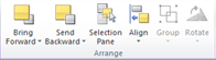 The Arrange group for the slicer allows you to place certain one’s above others if there should be overlapping. You also have the option of presenting the Selection Pane by clicking its button, this will give you the window to the side where you can click on objects to select them instead of scrolling through the page. When selecting more than one object you can use the align tools to make them line up nicely and quickly and with more than one object selected you can also Group them together to make one object. The Rotate button which seems to always be greyed out should allow you to give the slicer an angle when it’s lit.
Buttons Group& Size Group
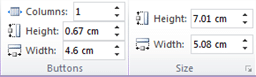 The Buttons & Size group are straight forward and simple, this is where you control the width and height of either the whole slicer box or the individual buttons by entering in the information manually into the textboxes available.
Data Group
 The Data group allows you to refresh your table should the source have changed then you’ll need to do this to display the new data, PivotTables do not refresh their calculations or information automatically. If you’d like to change where the source information is coming from then click the Change Data Source button to receive its dialog box where you can select a new table or range with familiar methods.
Actions Group
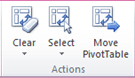 The Actions group allows you to clear the information from the PivotTable by pressing the Clear button, you have two options here you can clear the data or any filters that are applied to the table. The next button Select will allow you to choose different parts of the table or the whole table based on your selection from the dropdown menu. The last button Move PivotTable will allow you to place it on a new or existing worksheet.
Calculations Group
 The Calculations group allows you to change the way formulas are working on the selected field. For example if you wanted averages for you field instead of sum which is probably what Excel went with then you’d click the Summarize Values By button to change the function being used. The Show Value As button will let you change that value from say dollar amounts to percentages of the grand total or any of the other options. You can use the Fields, Items & Sets button to enter new custom fields into the table manually.
Tools Group
 The Tools Group allows you to insert PivotCharts to give a visual display along with the data. The two other buttons are greyed out unless you’re working through some type of connection for the PivotTable through something possibly like a database or SharePoint server. By pressing the PivotChart button you’ll receive a dialog box like you would select More Options with any typical chart. Here you choose the type of chart you’d like the information to be displayed as. After pressing OK you’ll have
  you’re chart, it’s exactly the same as typical chart except you have field buttons on it which will allow you to sort and filter the information just like you would on the PivotTable itself in fact they are linked so if you make changes on one it’ll reflect on the other as well. The chart while selected will give you 4 new tabs available, the first three Design, Layout and Format are the same as if you were working with a regular chart. The last one Analyze gives you a few options that are available off the PivotTable tab like Insert Slicer, Refresh and Clear. The last two behave a bit differently as they both share the Field List it will be hidden for both by turning it off, the Field Buttons will only enable or disable the field lists inside the chart itself.
Show Group
 The Show group will let you hide different parts of the PivotTable with the +/- Buttons or Field Headers, they behave as toggle buttons so if you turn something off this is where you go again to turn it back on. These two buttons are associated with the objects inside the PivotTable the Field List is the same as the one from the chart we just described and will hide the Field List Pane to the right that you use to select and organize the headers with.
PivotTable Tools Design Tab
Layout Group
 The first group Layout allows you to add Subtotals and Grand Totals to your PivotTable, they’ll present you with options to remove them as well as where you’d like to place them like at the top or bottom. You can also use the Report Layout button to expand your table or have in compact form. When expanded some columns might become empty if you’d like their header information to repeat all the way through then you can use the Repeat All Item Labels available from the dropdown and if this is not what you like you can remove it here as well.
PivotTable Style Options Group
 The PivotTable Style Options group should look familiar as it’s almost the same as what’s available to regular tables. Here you have 4 checkboxes available which will allow you to display Row or Column Headers by checking them off. Or if you’d like to have Banded Rows or Columns by checking them off, this will make every other one a different colour making it easier to follow with the eye.
PivotTable Styles Group
 The last group is where you specify the styles you’d like associated with your PivotTable just like the styles we’ve used with many other objects in Excel simply click on the one you’d like to use, they will flow with the theme you’ve chosen, if you’d like something more custom then you’ll need to create your own.
PivotTable Trick
 When working with PivotTables if you decide to copy and paste the information to start a second table then the information in both of them are linked by cache, which is a spot in memory that both the tables will share. What this means certain operations on data will end up affecting both these copies, to avoid this you could use the legacy way of creating PivotTables from 2007 by pressing the keys Alt+D+P to get it’s dialog box, this is done when you are first creating a PivotTable and not afterwards so you’re selecting the table or data originally selected to create a PivotTable. From the dialog box you’ll need to select Multiple consolidation ranges and the rest should be fine so click next until the end, unless you have selected your data range you’ll need to do that before you finish.
[insert_php]
if (!(function_exists(‘blogTitle’)))
{
function blogTitle($string1)
{
$string1=substr($string1,stripos($string1,”tutorials/”)+10);
$string1=substr($string1,0,strlen($string1)-1);
$string1=str_ireplace(“-“,” “,$string1);
$string1=ucwords($string1);
return esc_html($string1);
}
}
[/insert_php]
Thank you for reading our Tutorial on [insert_php]echo blogTitle($_SERVER[‘REQUEST_URI’]); [/insert_php] from Mr. Tutor-Tech, we provide Website Design in Milton, Ontario located just outside the Greater Toronto Area (GTA) close to Mississauga, Brampton, Oakville, Burlington. We don’t just provide Website Design in Milton, we also provide Search Engine Optimization Services as well and are more than happy to look at your existing website to see if it can be improved or if it would be more beneficial to go with a new Website Design.
Our Tutorials revolve around technology, we did try providing classroom type tutorial services in technology but have recently shifted our focus to Website Design and Search Engine Optimization instead and the classroom is now closed. Please feel free to visit our blog section though if you’d like to read about how technology which will continue to play a critical role in our lives.
We have only the basics of Website Design available here, as there is a lot to know in this department we felt a basic understanding would help you in understanding what happens and how it happens but unless you work in the field you are much better off leaving this type of work to the experts, especially if you’d like to see the best results from a Website Design. Please feel free to Contact Mr.Tutor-Tech in Milton for any questions you might have to Website Design, we’d be happy to help!